Python | GPCP | 趋势分析 | 气候态

写在前面

和之前类似的内容，只不过换了一下数据为GPCP月平均资料。主要还是简单的趋势分析以及气候态空间分布，将绘制方法这里调整为basemap，也算是温习一下basemap的绘图函数

GPCP（月平均资料）

对 1979 年至 2023 年月平均 GCPCP 降水数据进行了初步分析：

趋势
气候态年平均降水量
降水率的面积加权平均值
纬向平均降水量

数据

月平均 GPCP（全球降水气候学项目）数据融合了测量站、卫星和探空观测的降雨量，以估计 1979 年至今 2.5 度全球网格上的月降雨量。

数据地址为

https://climatedataguide.ucar.edu/climate-data/gpcp-monthly-global-precipitation-climatology-project 上找到。

空间趋势

数据读取

import numpy as np
import scipy.stats as stats
import datetime 
from netCDF4 import Dataset as netcdf # netcdf4-python module
from cartopy.mpl.ticker import  LongitudeFormatter,LatitudeFormatter
import matplotlib.pyplot as plt
from mpl_toolkits.basemap import Basemap
import matplotlib.dates as mdates
from matplotlib.dates import MonthLocator, WeekdayLocator, DateFormatter
import matplotlib.ticker as ticker
import xarray as xr
from matplotlib.pylab import rcParams
rcParams['figure.figsize'] = 15, 6
import warnings
warnings.simplefilter('ignore')
path = r'I:/precip.mon.mean.nc'
# 读取数据
ds = xr.open_dataset(path).sel(time=slice('1979-01-01', '2023-12-01'))
lons   = ds ['lon'][:]
lats   = ds ['lat'][:]
time   = ds ['time'][:]
pr     = ds ['precip'][:]ds

趋势计算

计算趋势并分析

将降水数据 pr.data 重塑为 (nt, ngrd) 的形状，其中 nt 是时间步数，ngrd 是网格点数。order=‘F’ 表示按列优先重塑
初始化两个空数组 pr_rate 和 pr_val，用于存储每个网格点的降水变化率和p值，并将它们的值设为 NaN
遍历每个网格点 i
提取该网格点的时间序列数据 y，并去除 NaN 值，得到 y0
创建一个与 y0 长度相同的线性空间 x
使用 stats.linregress 进行线性回归，计算斜率 slope、截距 intercept、相关系数 r_value、p值 p_value 和标准误差 std_err
将斜率乘以120（假设数据是月度数据，转换为每十年的变化率）并存储在 pr_rate 中
将p值存储在 pr_val 中

undef = -99999.0
pr.data[pr.data==undef] = np.nan
nt,nlat,nlon = pr.shape
ngrd = nlat*nlon
nt,nlat,nlon
pr_grd  = pr.data.reshape((nt, ngrd), order='F') 
pr_rate = np.empty((ngrd,1))
pr_rate[:,:] = np.nan
pr_val = np.empty((ngrd,1))
pr_val[:,:] = np.nanfor i in range(ngrd): print(i)y = pr_grd[:,i]  y0 = y[~np.isnan(y)]    x = np.linspace(1,len(y0), len(y0))slope, intercept, r_value, p_value, std_err = stats.linregress(x, y0)pr_rate[i,0] = slope*120.0  pr_val[i,0]  = p_value pr_rate = pr_rate.reshape((nlat,nlon), order='F')
pr_val  = pr_val.reshape((nlat,nlon), order='F')

使用basemap可视化空间趋势分布

plt.figure(figsize=(12,6),dpi=200)
m = Basemap(projection='cyl', llcrnrlon=min(lons), llcrnrlat=min(lats),urcrnrlon=max(lons), urcrnrlat=max(lats))x, y = m(*np.meshgrid(lons, lats))
clevs = np.linspace(-0.6, 0.6, 25)
cs = m.contourf(x, y, pr_rate.squeeze(), clevs, cmap='RdYlBu_r')
m.drawcoastlines()
m.drawparallels(np.arange(-90.,91.,30.), labels=[1,0,0,0], fontsize=10)
m.drawmeridians(np.arange(-180.,181.,60.), labels=[0,0,0,1], fontsize=10)
cb = m.colorbar(cs)
plt.title('GPCP  Changing Rate (mm/day/decade)', fontsize=16)sig_lats, sig_lons = np.where(pr_val < 0.05)
m.scatter(lons[sig_lons], lats[sig_lats], marker='o', color='k', s=1)
plt.show()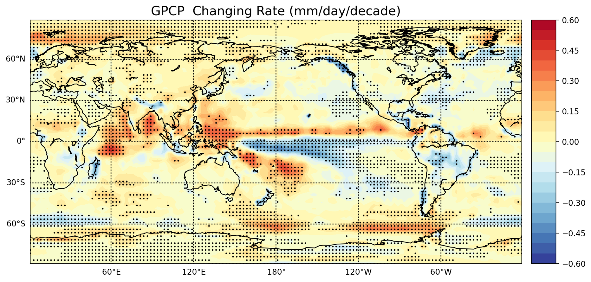

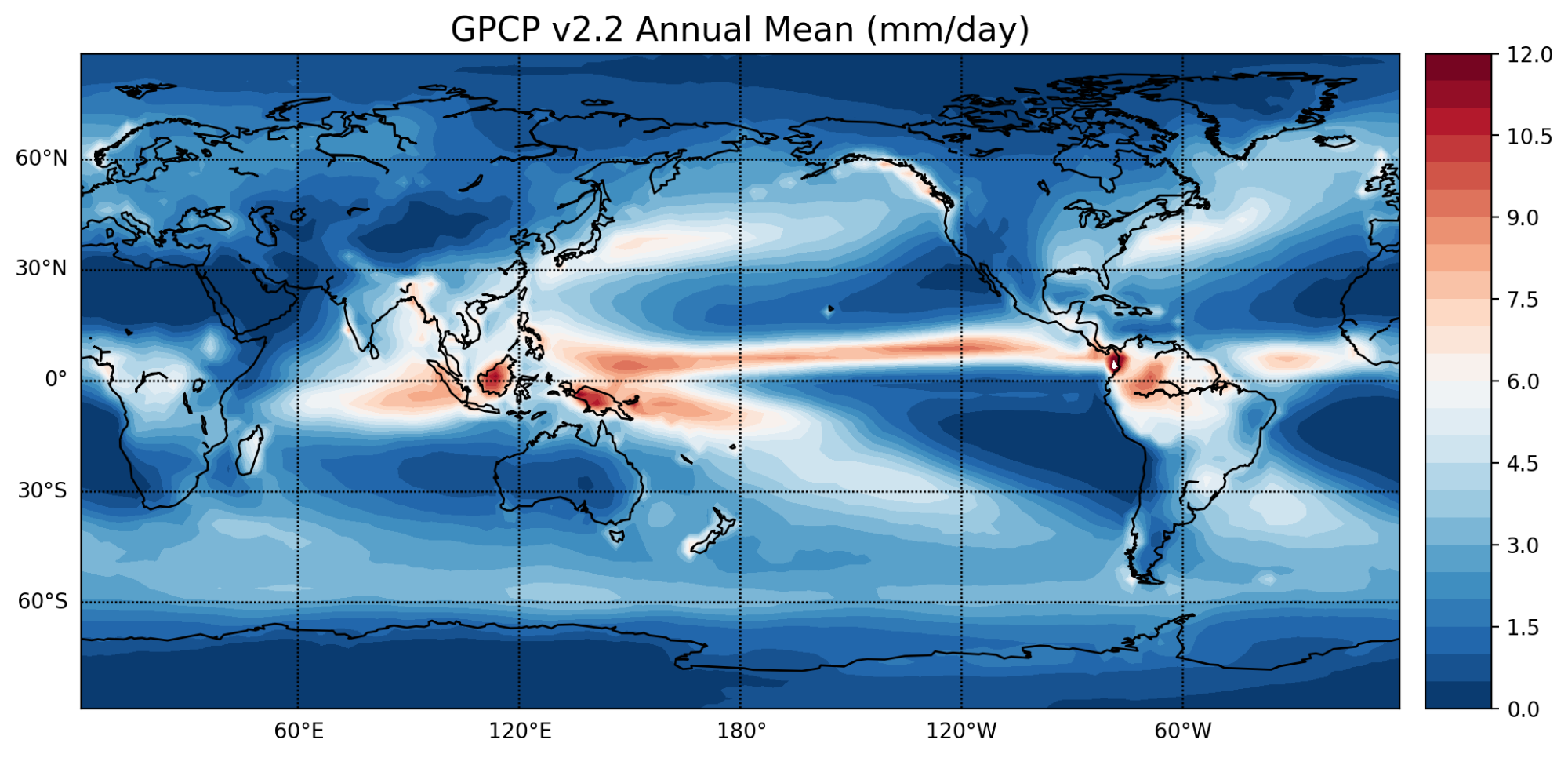
气候态平均

pr_ann_clm  = np.nanmean(pr, axis=0)
plt.figure(figsize=(12,6),dpi=200)
m = Basemap(projection='cyl', llcrnrlon=min(lons), llcrnrlat=min(lats),urcrnrlon=max(lons), urcrnrlat=max(lats))x, y = m(*np.meshgrid(lons, lats))
clevs = np.linspace(0.0, 12.0, 25)
cs = m.contourf(x, y, pr_ann_clm.squeeze(), clevs, cmap=plt.cm.RdBu_r)
m.drawcoastlines()
m.drawparallels(np.arange(-90.,91.,30.), labels=[1,0,0,0], fontsize=10)
m.drawmeridians(np.arange(-180.,181.,60.), labels=[0,0,0,1], fontsize=10)
cb = m.colorbar(cs)
plt.title('GPCP v2.2 Annual Mean (mm/day)', fontsize=16)

全球平均 | 纬向平均 | 经向平均

计算每个网格点的权重，权重是纬度的余弦值，用于加权平均。纬度越高，权重越小。
遍历每个时间步 it。
提取该时间步的降水数据 pone。
将数据中的 NaN 值掩盖，创建一个掩码数组 pone。
使用权重计算该时间步的加权平均降水量，并存储在 pr_glb_avg 中。

lonx, latx = np.meshgrid(lons, lats)
weights = np.cos(latx * np.pi / 180.)pr_glb_avg = np.zeros(nt)for it in np.arange(nt):pone = pr[it,:, :]pone = np.ma.masked_array(pone, mask=np.isnan(pone))pr_glb_avg[it] = np.average(pone, weights=weights) glb_avg = np.mean(pr_glb_avg)
print(glb_avg)
print(pr_glb_avg.shape)fig, ax = plt.subplots(1, 1, figsize=(15,6))ax.plot(time, pr_glb_avg, color='b', linewidth=2)ax.axhline(glb_avg, linewidth=2, color='r', label="Global areal mean: " + str(np.round(glb_avg*100)/100))
ax.legend()
ax.set_title('GPCP areal mean (1979-2023)', fontsize=16)
ax.set_xlabel('Month/Year #', fontsize=12)
ax.set_ylabel('Preicipitation [mm/day]', fontsize=12)
ax.set_ylim(2.4, 2.9)
ax.minorticks_on()
fig.autofmt_xdate()
ax.fmt_xdata = mdates.DateFormatter('%Y')

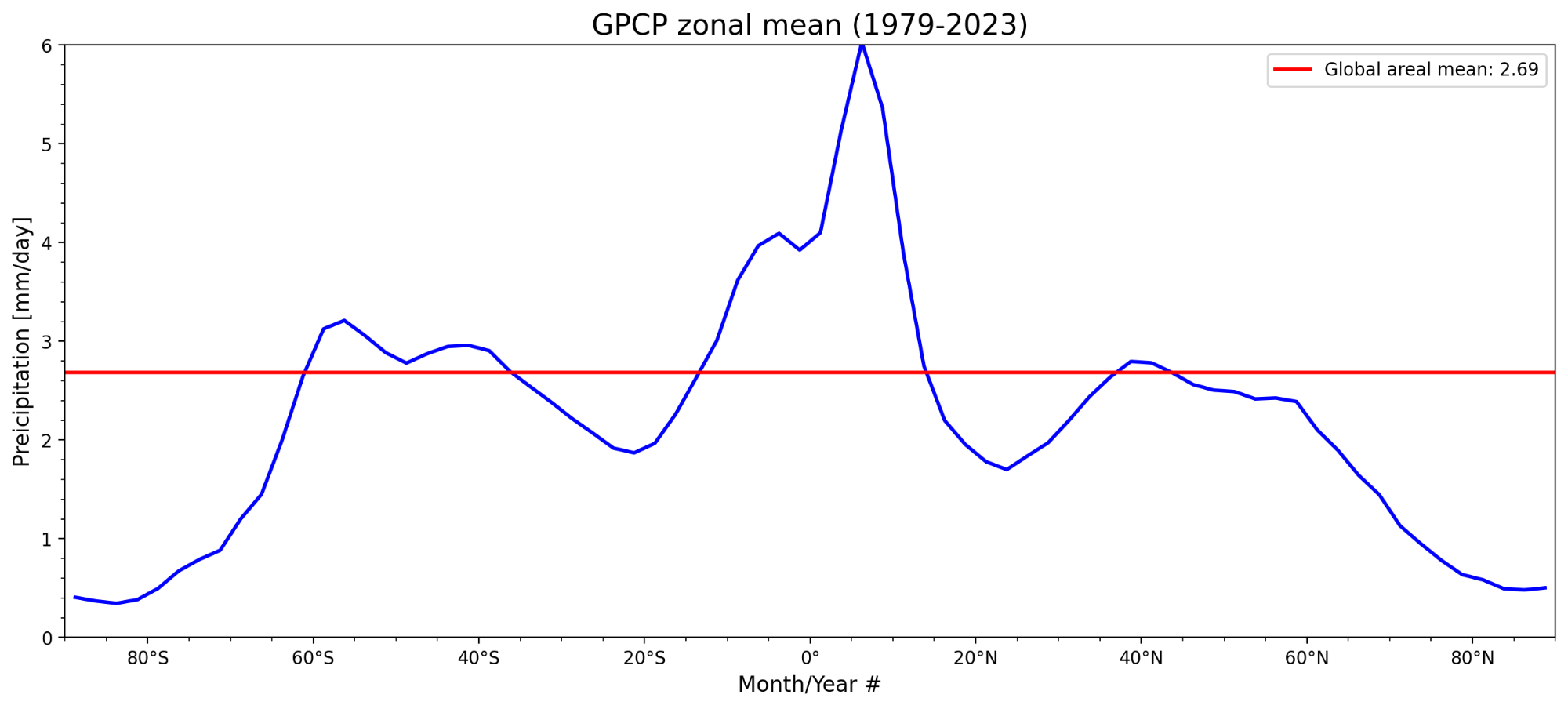
纬向平均

pr_ann_clm   = np.nanmean(pr, axis=0)
pr_ann_zonal = np.nanmean(pr_ann_clm, axis=1)
pr_ann_clm.shape
fig, ax = plt.subplots(1, 1, figsize=(15,6),dpi=200)ax.plot(lats, pr_ann_zonal, color='b', linewidth=2)ax.axhline(glb_avg, linewidth=2, color='r', label="Global areal mean: " + str(np.round(glb_avg*100)/100))
ax.legend()
ax.set_title('GPCP zonal mean (1979-2023)', fontsize=16)
ax.set_xlabel('Month/Year #', fontsize=12)
ax.set_ylabel('Preicipitation [mm/day]', fontsize=12)
ax.set_ylim(0.0, 6.0)
ax.set_xlim(-90, 90)
ax.xaxis.set_major_formatter(LatitudeFormatter())
ax.minorticks_on()

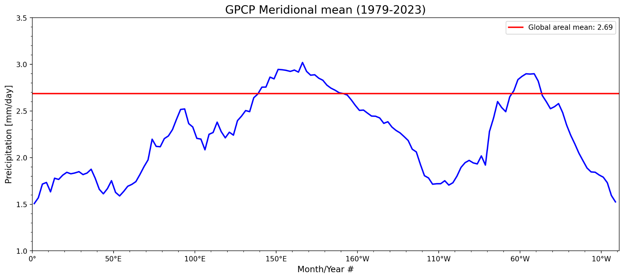
经向平均

pr_ann_mer = np.nanmean(pr_ann_clm, axis=0)
fig, ax = plt.subplots(1, 1, figsize=(15,6),dpi=200)
ax.plot(lons, pr_ann_mer, color='b', linewidth=2)
ax.axhline(glb_avg, linewidth=2, color='r', label="Global areal mean: " + str(np.round(glb_avg*100)/100))
ax.legend()
ax.set_title('GPCP Meridional mean (1979-2023)', fontsize=16)
ax.set_xlabel('Month/Year #', fontsize=12)
ax.set_ylabel('Preicipitation [mm/day]', fontsize=12)
ax.set_ylim(1, 3.5)
ax.set_xlim(0, 361)
ax.xaxis.set_major_formatter(LongitudeFormatter())
ax.minorticks_on()