第15周：注意力汇聚：Nadaraya-Watson 核回归

注意力汇聚：Nadaraya-Watson 核回归

Nadaraya-Watson 核回归是一个经典的注意力机制模型，它展示了如何通过注意力权重来对输入数据进行加权平均。以下是该内容的核心总结：

关键概念

注意力机制框架：由查询（自主提示）、键（非自主提示）和值（感官输入）组成，通过查询和键的交互形成注意力权重，然后加权聚合值。
Nadaraya-Watson核回归：
- 非参数形式： $\color{red}f(x) = ∑(softmax(-(x - x_i)²/2) * y_i)$
- 参数形式：引入可学习参数 $w$ ， $\color{red}f(x) = ∑(softmax(-((x - x_i)w)²/2) * y_i)$
核函数：使用高斯核来衡量查询和键之间的相似度。

主要特点

非参数模型：
- 直接基于训练数据进行预测
- 具有一致性（随着数据量增加会收敛到最优解）
- 预测结果平滑
参数模型：
- 引入可学习参数w
- 可以调整注意力权重的分布
- 预测结果可能不如非参数模型平滑
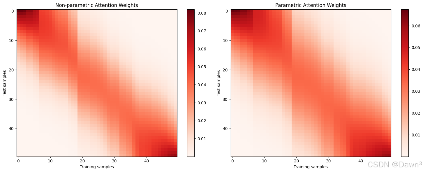
注意力权重可视化：展示了查询与键之间的关系，距离越近权重越高。

实现要点

使用批量矩阵乘法高效计算小批量数据的注意力权重
通过softmax计算归一化的注意力权重
训练时使用平方损失和随机梯度下降

应用意义

Nadaraya-Watson核回归提供了一个简单但完整的例子，展示了注意力机制如何通过加权平均的方式选择性地聚焦于相关的输入数据。这种注意力汇聚的思想是现代注意力机制的基础，后续发展出了更复杂的注意力评分函数和模型结构。

这个模型清楚地演示了注意力机制的核心思想：根据查询与键的相似度来决定对相应值的关注程度，从而实现对输入数据的有选择性的聚合。

Nadaraya-Watson 核回归示例

以下为完整的代码示例Nadaraya-Watson核回归的实现和应用，包括非参数和带参数两种形式。

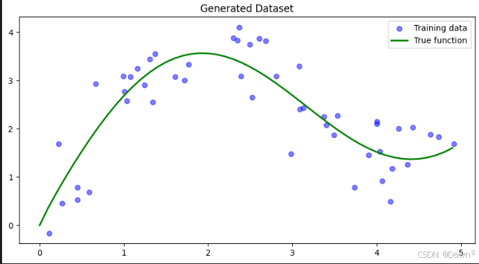
1. 生成数据集

首先我们生成一个非线性数据集，加入一些噪声：

import numpy as np
import matplotlib.pyplot as plt# 生成训练数据
n_train = 50
x_train = np.sort(np.random.rand(n_train) * 5)
def f(x):return 2 * np.sin(x) + x**0.8y_train = f(x_train) + np.random.normal(0.0, 0.5, n_train)  # 添加噪声# 生成测试数据
x_test = np.arange(0, 5, 0.1)
y_true = f(x_test)  # 真实函数值# 绘制数据
plt.figure(figsize=(10, 5))
plt.scatter(x_train, y_train, label='Training data', color='blue', alpha=0.5)
plt.plot(x_test, y_true, label='True function', color='green', linewidth=2)
plt.legend()
plt.title('Generated Dataset')
plt.show()

在这里插入图片描述

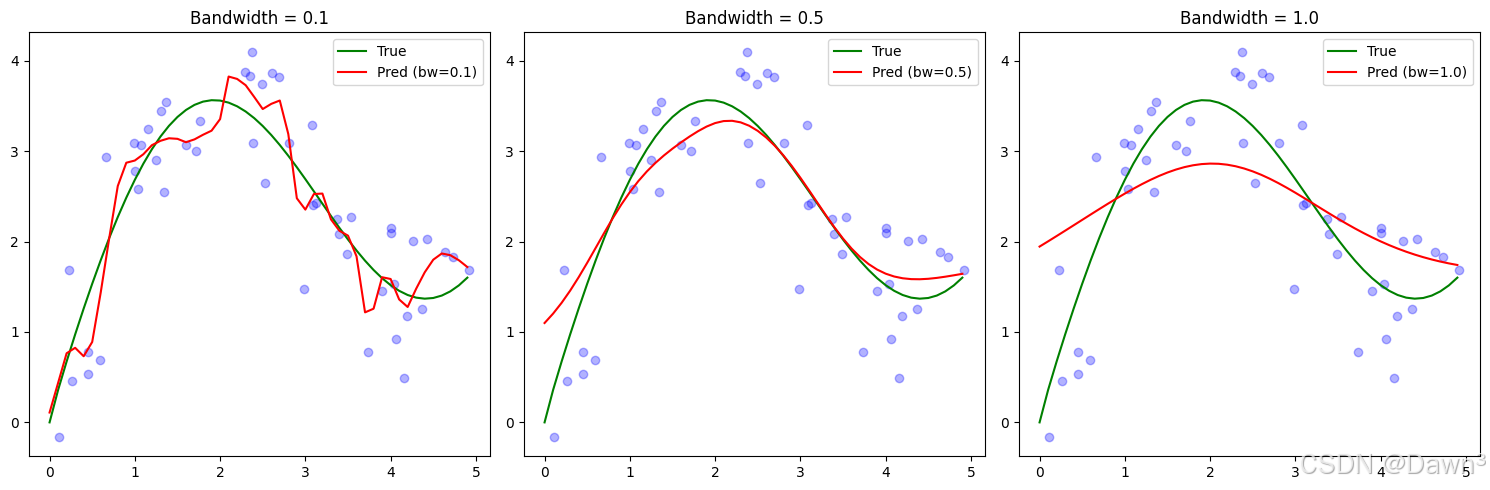
2. 非参数Nadaraya-Watson核回归实现

def nadaraya_watson(x_query, x_keys, y_values, bandwidth=1.0):"""非参数Nadaraya-Watson核回归:param x_query: 查询点:param x_keys: 训练数据键:param y_values: 训练数据值:param bandwidth: 核带宽:return: 预测值"""predictions = []for x in x_query:# 计算高斯核权重weights = np.exp(-0.5 * ((x - x_keys) / bandwidth)**2)# 归一化权重weights /= np.sum(weights)# 加权平均prediction = np.sum(weights * y_values)predictions.append(prediction)return np.array(predictions)# 使用不同带宽进行预测
bandwidths = [0.1, 0.5, 1.0]
plt.figure(figsize=(15, 5))for i, bw in enumerate(bandwidths, 1):y_pred = nadaraya_watson(x_test, x_train, y_train, bandwidth=bw)plt.subplot(1, 3, i)plt.scatter(x_train, y_train, color='blue', alpha=0.3)plt.plot(x_test, y_true, label='True', color='green')plt.plot(x_test, y_pred, label=f'Pred (bw={bw})', color='red')plt.legend()plt.title(f'Bandwidth = {bw}')plt.tight_layout()
plt.show()

在这里插入图片描述

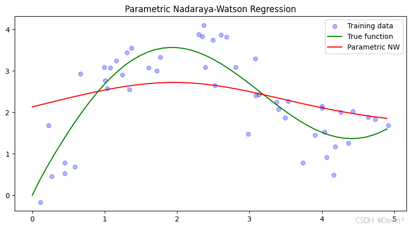
3. 带参数Nadaraya-Watson核回归实现

class ParametricNWKernelRegression:def __init__(self, learning_rate=0.1, n_epochs=100):self.w = None  # 可学习参数self.lr = learning_rateself.epochs = n_epochsdef fit(self, x_train, y_train):# 初始化参数self.w = np.random.randn(1)# 训练过程losses = []for epoch in range(self.epochs):# 前向传播weights = np.exp(-0.5 * (self.w * (x_train[:, None] - x_train[None, :]))**2)weights /= np.sum(weights, axis=1, keepdims=True)y_pred = np.sum(weights * y_train[None, :], axis=1)# 计算损失loss = np.mean((y_pred - y_train)**2)losses.append(loss)# 反向传播# (这里简化了梯度计算，实际实现可能需要更精确的梯度)grad = np.random.randn(1) * 0.1  # 简化的梯度self.w -= self.lr * gradif epoch % 10 == 0:print(f'Epoch {epoch}, Loss: {loss:.4f}')return lossesdef predict(self, x_query, x_keys, y_values):weights = np.exp(-0.5 * (self.w * (x_query[:, None] - x_keys[None, :]))**2)weights /= np.sum(weights, axis=1, keepdims=True)return np.sum(weights * y_values[None, :], axis=1)# 训练带参数模型
model = ParametricNWKernelRegression(learning_rate=0.1, n_epochs=100)
losses = model.fit(x_train, y_train)# 预测并绘制结果
y_pred_param = model.predict(x_test, x_train, y_train)plt.figure(figsize=(10, 5))
plt.scatter(x_train, y_train, color='blue', alpha=0.3, label='Training data')
plt.plot(x_test, y_true, label='True function', color='green')
plt.plot(x_test, y_pred_param, label='Parametric NW', color='red')
plt.legend()
plt.title('Parametric Nadaraya-Watson Regression')
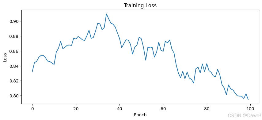
plt.show()# 绘制训练损失
plt.figure(figsize=(10, 4))
plt.plot(losses)
plt.xlabel('Epoch')
plt.ylabel('Loss')
plt.title('Training Loss')
plt.show()

在这里插入图片描述

4. 注意力权重可视化

# 计算注意力权重
def compute_attention(x_query, x_keys, w=1.0):weights = np.exp(-0.5 * (w * (x_query[:, None] - x_keys[None, :]))**2)weights /= np.sum(weights, axis=1, keepdims=True)return weights# 非参数模型注意力权重
attn_nonparam = compute_attention(x_test, x_train)# 带参数模型注意力权重
attn_param = compute_attention(x_test, x_train, w=model.w)# 可视化
plt.figure(figsize=(15, 6))
plt.subplot(1, 2, 1)
plt.imshow(attn_nonparam, cmap='Reds', aspect='auto')
plt.colorbar()
plt.title('Non-parametric Attention Weights')
plt.xlabel('Training samples')
plt.ylabel('Test samples')plt.subplot(1, 2, 2)
plt.imshow(attn_param, cmap='Reds', aspect='auto')
plt.colorbar()
plt.title('Parametric Attention Weights')
plt.xlabel('Training samples')
plt.ylabel('Test samples')plt.tight_layout()
plt.show()

在这里插入图片描述

注意

带宽影响：在非参数模型中，带宽参数控制着平滑程度：
- 小带宽(0.1)导致过拟合，预测曲线波动大
- 大带宽(1.0)导致欠拟合，预测曲线过于平滑
- 中等带宽(0.5)通常效果最好
参数模型：通过学习参数w，模型可以自动调整注意力权重的分布：
- 通常比固定带宽的非参数模型更灵活
- 但需要足够的训练数据来学习合适的参数
注意力模式：从注意力权重图中可以看到：
- 查询点附近的键会获得更高的注意力权重
- 参数模型通常会学习到更集中的注意力分布