第1讲、#PyTorch教学环境搭建与Tensor基础操作详解

引言

PyTorch是当前深度学习领域最流行的框架之一，因其动态计算图和直观的API而备受开发者青睐。本文将从零开始介绍PyTorch的环境搭建与基础操作，适合各种平台的用户和深度学习初学者。

1. 安装和环境搭建

macOS (Apple Silicon)

对于Mac M1/M2/M3用户，PyTorch现已支持Metal加速，可直接通过pip安装：

pip install torch torchvision torchaudio

Windows/Linux/Intel Mac

通过pip安装（CPU版本）：

pip install torch torchvision torchaudio

通过pip安装（CUDA版本，以CUDA 11.8为例）：

pip install torch torchvision torchaudio --index-url https://download.pytorch.org/whl/cu118

Conda环境（推荐）

使用Conda可以更好地管理依赖：

# 创建新的conda环境
conda create -n pytorch python=3.10
conda activate pytorch# 安装PyTorch（CPU版本）
conda install pytorch torchvision torchaudio -c pytorch# 或GPU版本（以CUDA 11.8为例）
conda install pytorch torchvision torchaudio pytorch-cuda=11.8 -c pytorch -c nvidia

验证安装

安装完成后，可以通过以下代码验证是否安装成功：

import torchprint(torch.__version__)# GPU检查（对于NVIDIA GPU）
print("CUDA可用:", torch.cuda.is_available())
if torch.cuda.is_available():print("CUDA设备数量:", torch.cuda.device_count())print("CUDA设备名称:", torch.cuda.get_device_name(0))# Apple Silicon检查
if hasattr(torch.backends, 'mps'):print("MPS可用:", torch.backends.mps.is_available())print("MPS内置:", torch.backends.mps.is_built())

2. 什么是Tensor（张量）？

Tensor（张量）是PyTorch的核心数据结构，它是一种多维数组，可以看作是标量（0维张量）、向量（1维张量）、矩阵（2维张量）的推广到任意维度的数学对象。简单来说，Tensor是一个可以存储和操作多维数据的容器。

2.1 Tensor的作用

Tensor在深度学习中扮演着至关重要的角色：

1. 数据表示：用于表示各种类型的数据，如图像（3D或4D张量）、文本（序列的数值表示）、音频信号等。

2. 参数存储：神经网络的权重、偏置等参数都以Tensor形式存储。

3. 梯度计算：PyTorch中的Tensor支持自动微分，能够自动追踪计算历史并计算梯度，这是深度学习训练的基础。

4. 数学运算：提供丰富的数学运算支持，如加减乘除、矩阵乘法、卷积等，使复杂的数学运算变得简单。

5. GPU加速：可以无缝地在CPU和GPU之间移动，利用GPU进行并行计算，大幅提升运算速度。

2.2 Tensor的展现形式

Tensor可以有多种展现形式，根据其维度而定：

1. 0维张量（标量）：单个数值

   scalar = torch.tensor(42)
   print(scalar)  # tensor(42)
   print(scalar.shape)  # torch.Size([])
   

2. 1维张量（向量）：数值序列

   vector = torch.tensor([1, 2, 3, 4])
   print(vector)  # tensor([1, 2, 3, 4])
   print(vector.shape)  # torch.Size([4])
   

3. 2维张量（矩阵）：数值表格

   matrix = torch.tensor([[1, 2], [3, 4], [5, 6]])
   print(matrix)
   # tensor([[1, 2],
   #         [3, 4],
   #         [5, 6]])
   print(matrix.shape)  # torch.Size([3, 2]) - 3行2列
   

4. 3维张量：可以想象为多个矩阵堆叠在一起，常用于表示图像（通道、高度、宽度）

   tensor_3d = torch.rand(3, 4, 5)  # 3个4行5列的矩阵
   print(tensor_3d.shape)  # torch.Size([3, 4, 5])
   

5. 4维及以上张量：更高维度的数据结构，例如批量图像（批量大小、通道数、高度、宽度）

   batch_images = torch.rand(32, 3, 224, 224)  # 32张3通道224x224的图像
   print(batch_images.shape)  # torch.Size([32, 3, 224, 224])
   

2.3 Tensor的可视化表示

为帮助理解，我们可以将不同维度的Tensor视觉化表示：

• 0维张量：一个点
• 1维张量：一条线（数据点沿一个轴排列）
• 2维张量：一个平面（数据点按行列排列）
• 3维张量：一个立方体（如RGB图像中的三个颜色通道）
• 4维张量：可以视为多个3D对象的集合（如一批图像）

2.4 Tensor与NumPy数组的关系

PyTorch的Tensor与NumPy的ndarray非常相似，两者可以方便地相互转换：

import torch
import numpy as np# NumPy数组转Tensor
numpy_array = np.array([1, 2, 3])
tensor = torch.from_numpy(numpy_array)# Tensor转NumPy数组
tensor = torch.tensor([4, 5, 6])
numpy_array = tensor.numpy()

主要区别在于PyTorch的Tensor支持GPU加速和自动微分，这使其特别适合深度学习任务。

3. Tensor基础操作

3.1 创建不同类型的Tensor

import torch# 创建一个1维Tensor
a = torch.tensor([1, 2, 3])
print("1维 Tensor:", a)# 创建一个2维Tensor
b = torch.tensor([[1, 2], [3, 4]])
print("2维 Tensor:\n", b)# 创建float类型的Tensor
c = torch.tensor([1.0, 2.0, 3.0], dtype=torch.float32)
print("float Tensor:", c)# 创建指定shape的零矩阵
d = torch.zeros((2, 3))
print("零矩阵:\n", d)# 创建指定shape的随机矩阵
e = torch.rand((2, 2))
print("随机Tensor:\n", e)

3.2 Tensor基本运算

PyTorch支持各种数学运算，使用方式直观简洁：

x = torch.tensor([1, 2, 3])
y = torch.tensor([9, 8, 7])# 加法
print("加法:", x + y)  # 输出: tensor([10, 10, 10])# 减法
print("减法:", x - y)  # 输出: tensor([-8, -6, -4])# 乘法(逐元素)
print("乘法:", x * y)  # 输出: tensor([9, 16, 21])# 除法
print("除法:", x / y)  # 输出: tensor([0.1111, 0.2500, 0.4286])# 矩阵运算（点乘）
dot_product = torch.dot(x.float(), y.float())
print("点乘结果:", dot_product)  # 输出: tensor(46.)

3.3 Tensor形状操作（reshape）

改变Tensor的形状是深度学习中的常见操作：

# 创建一个4x4的随机Tensor
z = torch.rand((4, 4))
print("原始形状:\n", z)# reshape成16x1
z_reshaped = z.view(16, 1)
print("reshape后的形状:\n", z_reshaped)# reshape回2x8
z_reshaped2 = z.view(2, 8)
print("再reshape:\n", z_reshaped2)

4. 在CPU和GPU之间移动Tensor

4.1 检查设备

在使用GPU加速前，需要检查设备可用性：

# 通用检测和设备选择
if torch.cuda.is_available():device = torch.device("cuda")
elif hasattr(torch.backends, 'mps') and torch.backends.mps.is_available():device = torch.device("mps")
else:device = torch.device("cpu")print("当前使用设备:", device)

4.2 Tensor在设备之间转移

将Tensor在CPU和GPU之间转移是通过.to()方法实现的：

# 创建一个Tensor
tensor_cpu = torch.ones((3, 3))
print("CPU上的Tensor:\n", tensor_cpu)# 将Tensor移动到GPU
tensor_gpu = tensor_cpu.to(device)
print("GPU上的Tensor:\n", tensor_gpu)# 再移回CPU
tensor_back = tensor_gpu.to('cpu')
print("回到CPU的Tensor:\n", tensor_back)

总结

通过本文，我们学习了：

• 在不同平台上安装并配置PyTorch环境
• 理解Tensor的本质、作用和展现形式
• Tensor的创建、基本运算和形状操作
• 如何利用GPU（包括NVIDIA CUDA和Apple Silicon的MPS）加速功能

掌握这些基础知识后，你就可以开始构建和训练简单的深度学习模型了。下一篇文章将介绍神经网络的构建和训练基础。

5. 实战案例：使用Streamlit可视化Tensor

为了更直观地理解Tensor，我们可以使用Streamlit创建一个简单的Web应用来可视化不同维度的Tensor。下面是一个完整的示例代码：

5.1 安装所需包

首先，安装必要的包：

pip install streamlit numpy torch matplotlib plotly

5.2 创建Streamlit应用

将以下代码保存为tensor_visualizer.py：

import streamlit as st
import torch
import numpy as np
import matplotlib.pyplot as plt
import plotly.graph_objects as go
import plotly.express as pxst.set_page_config(page_title="PyTorch Tensor可视化", layout="wide")
st.title("PyTorch Tensor可视化工具")# 侧边栏选项
st.sidebar.header("Tensor设置")
tensor_dim = st.sidebar.radio("选择Tensor维度", [0, 1, 2, 3, 4], index=2)# 根据维度提供不同选项
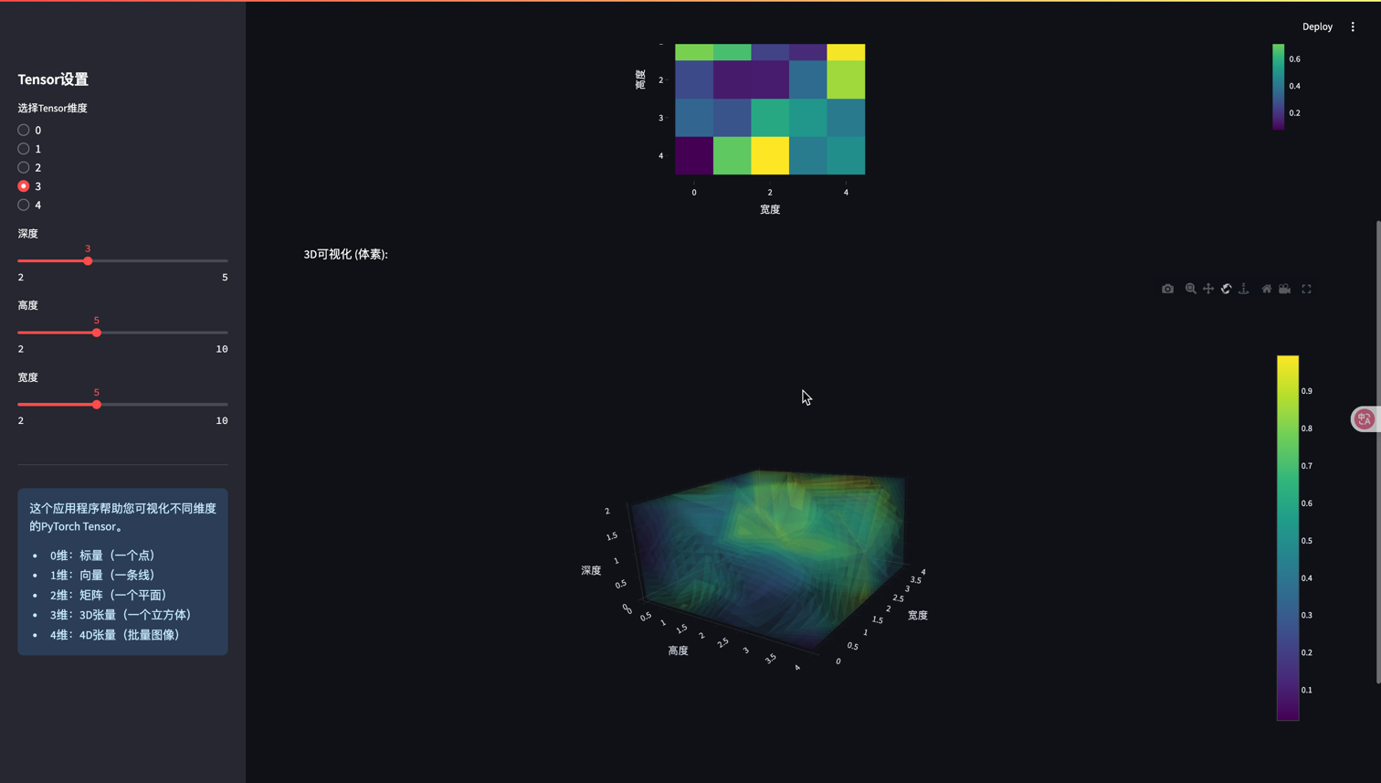
if tensor_dim == 0:  # 标量scalar_value = st.sidebar.slider("标量值", -10.0, 10.0, 5.0, 0.1)st.header("0维Tensor (标量)")tensor = torch.tensor(scalar_value)st.code(f"tensor = torch.tensor({scalar_value})")st.write(f"值: {tensor.item()}")st.write(f"形状: {tensor.shape}")# 可视化st.write("可视化: 一个点")fig, ax = plt.subplots(figsize=(3, 3))ax.scatter([0], [0], s=100, c=[scalar_value], cmap='viridis')ax.set_xlim(-1, 1)ax.set_ylim(-1, 1)ax.set_xticks([])ax.set_yticks([])st.pyplot(fig)elif tensor_dim == 1:  # 向量vector_size = st.sidebar.slider("向量大小", 2, 20, 10)vector_type = st.sidebar.selectbox("向量类型", ["随机", "线性", "正弦波"])st.header("1维Tensor (向量)")if vector_type == "随机":tensor = torch.rand(vector_size)elif vector_type == "线性":tensor = torch.linspace(0, 10, vector_size)else:  # 正弦波tensor = torch.sin(torch.linspace(0, 6.28, vector_size))st.code(f"tensor.shape = {tensor.shape}")st.write("Tensor值:")st.write(tensor)# 可视化st.write("可视化:")fig, ax = plt.subplots(figsize=(10, 4))ax.plot(tensor.numpy(), marker='o')ax.set_title("1维Tensor可视化")ax.set_xlabel("索引")ax.set_ylabel("值")ax.grid(True)st.pyplot(fig)elif tensor_dim == 2:  # 矩阵rows = st.sidebar.slider("行数", 2, 10, 5)cols = st.sidebar.slider("列数", 2, 10, 5)tensor_type = st.sidebar.selectbox("矩阵类型", ["随机", "单位矩阵", "对角矩阵"])st.header("2维Tensor (矩阵)")if tensor_type == "随机":tensor = torch.rand(rows, cols)elif tensor_type == "单位矩阵":tensor = torch.eye(max(rows, cols))[:rows, :cols]else:  # 对角矩阵tensor = torch.diag(torch.linspace(1, min(rows, cols), min(rows, cols)))if rows > cols:tensor = torch.cat([tensor, torch.zeros(rows - cols, cols)], dim=0)elif cols > rows:tensor = torch.cat([tensor, torch.zeros(rows, cols - rows)], dim=1)st.code(f"tensor.shape = {tensor.shape}")st.write("Tensor值:")st.write(tensor)# 可视化为热力图st.write("可视化:")fig = px.imshow(tensor.numpy(), labels=dict(x="列", y="行", color="值"),color_continuous_scale='viridis')fig.update_layout(width=600, height=500)st.plotly_chart(fig)elif tensor_dim == 3:  # 3D Tensordepth = st.sidebar.slider("深度", 2, 5, 3)height = st.sidebar.slider("高度", 2, 10, 5)width = st.sidebar.slider("宽度", 2, 10, 5)st.header("3维Tensor")tensor = torch.rand(depth, height, width)st.code(f"tensor.shape = {tensor.shape}")# 展示每个深度层st.write("每个深度的切片可视化:")tabs = st.tabs([f"切片 {i}" for i in range(depth)])for i, tab in enumerate(tabs):with tab:fig = px.imshow(tensor[i].numpy(),labels=dict(x="宽度", y="高度", color="值"),color_continuous_scale='viridis')fig.update_layout(width=500, height=400)st.plotly_chart(fig)# 3D可视化st.write("3D可视化 (体素):")# 创建网格X, Y, Z = np.mgrid[0:depth, 0:height, 0:width]values = tensor.numpy().flatten()fig = go.Figure(data=go.Volume(x=X.flatten(),y=Y.flatten(),z=Z.flatten(),value=values,opacity=0.1,surface_count=15,colorscale='viridis'))fig.update_layout(scene=dict(xaxis_title='深度', yaxis_title='高度', zaxis_title='宽度'),width=700, height=700)st.plotly_chart(fig)elif tensor_dim == 4:  # 4D Tensorbatch = st.sidebar.slider("批量大小", 1, 5, 2)channels = st.sidebar.slider("通道数", 1, 3, 3)height = st.sidebar.slider("高度", 4, 12, 8)width = st.sidebar.slider("宽度", 4, 12, 8)st.header("4维Tensor (批量图像)")tensor = torch.rand(batch, channels, height, width)st.code(f"tensor.shape = {tensor.shape}")st.write(f"这个Tensor可以表示{batch}张{channels}通道的{height}x{width}图像")# 可视化每个批次的图像batch_tabs = st.tabs([f"批次 {i}" for i in range(batch)])for b, batch_tab in enumerate(batch_tabs):with batch_tab:if channels == 3:# 针对RGB图像的特殊处理img = tensor[b].permute(1, 2, 0).numpy()  # 转换为HWC格式st.image(img, caption=f"批次 {b} 的RGB图像", use_column_width=True)else:# 展示每个通道channel_tabs = st.tabs([f"通道 {i}" for i in range(channels)])for c, channel_tab in enumerate(channel_tabs):with channel_tab:fig = px.imshow(tensor[b, c].numpy(),color_continuous_scale='viridis')fig.update_layout(width=400, height=400)st.plotly_chart(fig)# 添加信息部分
st.sidebar.markdown("---")
st.sidebar.info("""
这个应用程序帮助您可视化不同维度的PyTorch Tensor。
- 0维：标量（一个点）
- 1维：向量（一条线）
- 2维：矩阵（一个平面）
- 3维：3D张量（一个立方体）
- 4维：4D张量（批量图像）
""")# 添加代码说明
with st.expander("如何运行这个应用"):st.code("""
# 保存代码为tensor_visualizer.py后运行:
streamlit run tensor_visualizer.py""")

5.3 运行应用

使用以下命令运行应用：

streamlit run tensor_visualizer.py

5.4 应用功能

该应用允许用户：

1. 选择Tensor维度：从0维（标量）到4维（批量图像）
2. 调整Tensor参数：根据维度调整大小和类型
3. 直观可视化：生成适合每种维度的可视化效果
   • 0维：点
   • 1维：线图
   • 2维：热力图
   • 3维：三维体素图和切片
   • 4维：多通道图像

5.5 案例说明

通过这个Streamlit应用，您可以：

• 直观理解不同维度Tensor的概念
• 尝试修改参数，观察张量的变化
• 学习如何在Python中操作和可视化Tensor

这个应用程序是学习PyTorch Tensor的绝佳辅助工具，可以帮助初学者更好地理解深度学习中张量的表示方式。