Transformer 模型的 PyTorch 实现

Google 2017年的论文 Attention is all you need 阐释了什么叫做大道至简！该论文提出了Transformer模型，完全基于Attention mechanism，抛弃了传统的RNN和CNN。

我们根据论文的结构图，一步一步使用 PyTorch实现这个Transformer模型。

Transformer架构

首先看一下transformer的结构图：

解释一下这个结构图。首先，Transformer模型也是使用经典的encoer-decoder架构，由encoder和decoder两部分组成。

上图的左半边用Nx框出来的，就是我们的encoder的一层。encoder一共有6层这样的结构。

上图的右半边用Nx框出来的，就是我们的decoder的一层。decoder一共有6层这样的结构。

输入序列经过word embedding和positional encoding相加后，输入到encoder。

输出序列经过word embedding和positional encoding相加后，输入到decoder。

最后，decoder输出的结果，经过一个线性层，然后计算softmax。

word embedding和positional encoding我后面会解释。我们首先详细地分析一下encoder和decoder的每一层是怎么样的。

Encoder

encoder由6层相同的层组成，每一层分别由两部分组成：

• 第一部分是一个multi-head self-attention mechanism
• 第二部分是一个position-wise feed-forward network，是一个全连接层

两个部分，都有一个 残差连接(residual connection)，然后接着一个Layer Normalization。

如果你是一个新手，你可能会问：

• multi-head self-attention 是什么呢？
• 参差结构是什么呢？
• Layer Normalization又是什么？

这些问题我们在后面会一一解答。

Decoder

和encoder类似，decoder由6个相同的层组成，每一个层包括以下3个部分：

• 第一个部分是multi-head self-attention mechanism
• 第二部分是multi-head context-attention mechanism
• 第三部分是一个position-wise feed-forward network

还是和encoder类似，上面三个部分的每一个部分，都有一个残差连接，后接一个Layer Normalization。

但是，decoder出现了一个新的东西multi-head context-attention mechanism。这个东西其实也不复杂，理解了multi-head self-attention你就可以理解multi-head context-attention。这个我们后面会讲解。

Attention机制

在讲清楚各种attention之前，我们得先把attention机制说清楚。

通俗来说，attention是指，对于某个时刻的输出y，它在输入x上各个部分的注意力。这个注意力实际上可以理解为权重。

attention机制也可以分成很多种。Attention? Attention! 一问有一张比较全面的表格：

Figure 2. a summary table of several popular attention mechanisms.

上面第一种additive attention你可能听过。以前我们的seq2seq模型里面，使用attention机制，这种**加性注意力(additive attention)**用的很多。Google的项目 tensorflow/nmt里面使用的attention就是这种。

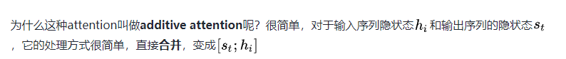
但是我们的transformer模型使用的不是这种attention机制，使用的是另一种，叫做乘性注意力(multiplicative attention)。

那么这种乘性注意力机制是怎么样的呢？从上表中的公式也可以看出来：两个隐状态进行点积！

Self-attention是什么？

到这里就可以解释什么是self-attention了。

所谓self-attention实际上就是，输出序列就是输入序列！因此，计算自己的attention得分，就叫做self-attention！

Context-attention是什么？

知道了self-attention，那你肯定猜到了context-attention是什么了：它是encoder和decoder之间的attention！所以，你也可以称之为encoder-decoder attention!

context-attention一词并不是本人原创，有些文章或者代码会这样描述，我觉得挺形象的，所以在此沿用这个称呼。其他文章可能会有其他名称，但是不要紧，我们抓住了重点即可，那就是两个不同序列之间的attention，与self-attention相区别。

不管是self-attention还是context-attention，它们计算attention分数的时候，可以选择很多方式，比如上面表中提到的：

• additive attention
• local-base
• general
• dot-product
• scaled dot-product

那么我们的Transformer模型，采用的是哪种呢？答案是：scaled dot-product attention。

Scaled dot-product attention是什么？

论文Attention is all you need里面对于attention机制的描述是这样的：

An attention function can be described as a query and a set of key-value pairs to an output, where the query, keys, values, and output are all vectors. The output is computed as a weighted sum of the values, where the weight assigned to each value is computed by a compatibility of the query with the corresponding key.

这句话描述得很清楚了。翻译过来就是：通过确定Q和K之间的相似程度来选择V！

用公式来描述更加清晰：

论文也提供了一张很清晰的结构图，供大家参考：

Figure 3. Scaled dot-product attention architecture.

首先说明一下我们的K、Q、V是什么：

• 在encoder的self-attention中，Q、K、V都来自同一个地方（相等），他们是上一层encoder的输出。对于第一层encoder，它们就是word embedding和positional encoding相加得到的输入。
• 在decoder的self-attention中，Q、K、V都来自于同一个地方（相等），它们是上一层decoder的输出。对于第一层decoder，它们就是word embedding和positional encoding相加得到的输入。但是对于decoder，我们不希望它能获得下一个time step（即将来的信息），因此我们需要进行sequence masking。
• 在encoder-decoder attention中，Q来自于decoder的上一层的输出，K和V来自于encoder的输出，K和V是一样的。
  

上面scaled dot-product attention和decoder的self-attention都出现了masking这样一个东西。那么这个mask到底是什么呢？这两处的mask操作是一样的吗？这个问题在后面会有详细解释。

Scaled dot-product attention的实现

咱们先把scaled dot-product attention实现了吧。代码如下：

复制代码import torch
import torch.nn as nnclass ScaledDotProductAttention(nn.Module):"""Scaled dot-product attention mechanism."""def __init__(self, attention_dropout=0.0):super(ScaledDotProductAttention, self).__init__()self.dropout = nn.Dropout(attention_dropout)self.softmax = nn.Softmax(dim=2)def forward(self, q, k, v, scale=None, attn_mask=None):"""前向传播.Args:q: Queries张量，形状为[B, L_q, D_q]k: Keys张量，形状为[B, L_k, D_k]v: Values张量，形状为[B, L_v, D_v]，一般来说就是kscale: 缩放因子，一个浮点标量attn_mask: Masking张量，形状为[B, L_q, L_k]Returns:上下文张量和attetention张量"""attention = torch.bmm(q, k.transpose(1, 2))if scale:attention = attention * scaleif attn_mask:# 给需要mask的地方设置一个负无穷attention = attention.masked_fill_(attn_mask, -np.inf)# 计算softmaxattention = self.softmax(attention)# 添加dropoutattention = self.dropout(attention)# 和V做点积context = torch.bmm(attention, v)return context, attention

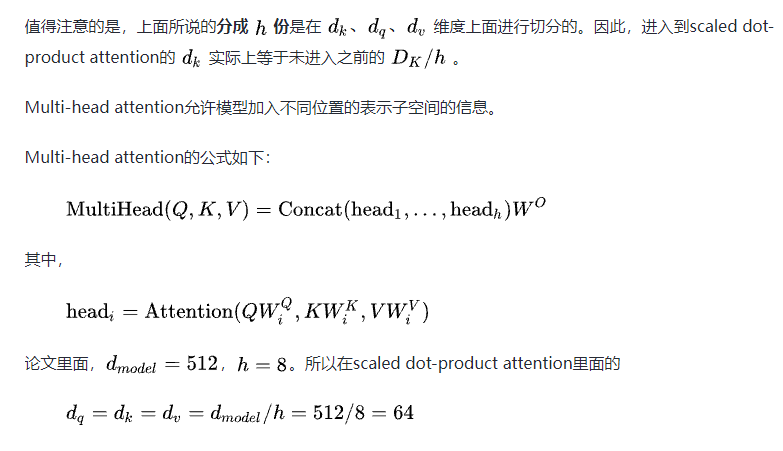
Multi-head attention又是什么呢？

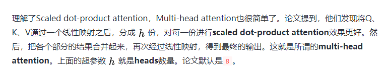
下面是multi-head attention的结构图：

Figure 4: Multi-head attention architecture.

Multi-head attention的实现

相信大家已经理清楚了multi-head attention，那么我们来实现它吧。代码如下：

复制代码import torch
import torch.nn as nnclass MultiHeadAttention(nn.Module):def __init__(self, model_dim=512, num_heads=8, dropout=0.0):super(MultiHeadAttention, self).__init__()self.dim_per_head = model_dim // num_headsself.num_heads = num_headsself.linear_k = nn.Linear(model_dim, self.dim_per_head * num_heads)self.linear_v = nn.Linear(model_dim, self.dim_per_head * num_heads)self.linear_q = nn.Linear(model_dim, self.dim_per_head * num_heads)self.dot_product_attention = ScaledDotProductAttention(dropout)self.linear_final = nn.Linear(model_dim, model_dim)self.dropout = nn.Dropout(dropout)# multi-head attention之后需要做layer normself.layer_norm = nn.LayerNorm(model_dim)def forward(self, key, value, query, attn_mask=None):# 残差连接residual = querydim_per_head = self.dim_per_headnum_heads = self.num_headsbatch_size = key.size(0)# linear projectionkey = self.linear_k(key)value = self.linear_v(value)query = self.linear_q(query)# split by headskey = key.view(batch_size * num_heads, -1, dim_per_head)value = value.view(batch_size * num_heads, -1, dim_per_head)query = query.view(batch_size * num_heads, -1, dim_per_head)if attn_mask:attn_mask = attn_mask.repeat(num_heads, 1, 1)# scaled dot product attentionscale = (key.size(-1) // num_heads) ** -0.5context, attention = self.dot_product_attention(query, key, value, scale, attn_mask)# concat headscontext = context.view(batch_size, -1, dim_per_head * num_heads)# final linear projectionoutput = self.linear_final(context)# dropoutoutput = self.dropout(output)# add residual and norm layeroutput = self.layer_norm(residual + output)return output, attention

上面的代码终于出现了Residual connection和Layer normalization。我们现在来解释它们。

Residual connection是什么？

残差连接其实很简单！给你看一张示意图你就明白了：

Figure 5. Residual connection.

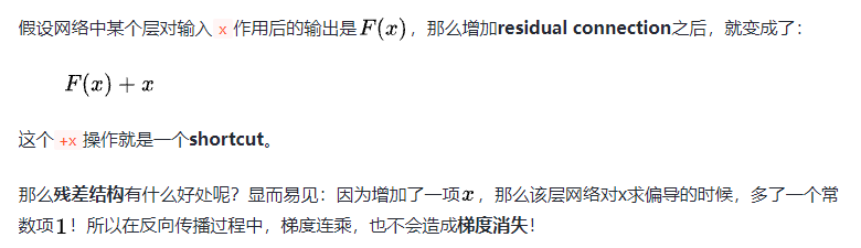
所以，代码实现residual connection很非常简单：

复制代码def residual(sublayer_fn,x):return sublayer_fn(x)+x

文章开始的transformer架构图中的Add & Norm中的Add也就是指的这个shortcut。

至此，residual connection的问题理清楚了。更多关于残差网络的介绍可以看文末的参考文献。

Layer normalization是什么？

GRADIENTS, BATCH NORMALIZATION AND LAYER NORMALIZATION一文对normalization有很好的解释：

Normalization有很多种，但是它们都有一个共同的目的，那就是把输入转化成均值为0方差为1的数据。我们在把数据送入激活函数之前进行normalization（归一化），因为我们不希望输入数据落在激活函数的饱和区。

说到normalization，那就肯定得提到Batch Normalization。BN在CNN等地方用得很多。

BN的主要思想就是：在每一层的每一批数据上进行归一化。

我们可能会对输入数据进行归一化，但是经过该网络层的作用后，我们的的数据已经不再是归一化的了。随着这种情况的发展，数据的偏差越来越大，我的反向传播需要考虑到这些大的偏差，这就迫使我们只能使用较小的学习率来防止梯度消失或者梯度爆炸。

BN的具体做法就是对每一小批数据，在批这个方向上做归一化。如下图所示：

Figure 6. Batch normalization example.(From theneuralperspective.com)

可以看到，右半边求均值是沿着数据批量N的方向进行的！

Batch normalization的计算公式如下：

具体的实现可以查看上图的链接文章。

说完Batch normalization，就该说说咱们今天的主角Layer normalization。

那么什么是Layer normalization呢？:它也是归一化数据的一种方式，不过LN是在每一个样本上计算均值和方差，而不是BN那种在批方向计算均值和方差！

下面是LN的示意图：

Figure 7. Layer normalization example.

和上面的BN示意图一比较就可以看出二者的区别啦！

下面看一下LN的公式，也BN十分相似：

Layer normalization的实现

复制代码import torch
import torch.nn as nnclass LayerNorm(nn.Module):"""实现LayerNorm。其实PyTorch已经实现啦，见nn.LayerNorm。"""def __init__(self, features, epsilon=1e-6):"""Init.Args:features: 就是模型的维度。论文默认512epsilon: 一个很小的数，防止数值计算的除0错误"""super(LayerNorm, self).__init__()# alphaself.gamma = nn.Parameter(torch.ones(features))# betaself.beta = nn.Parameter(torch.zeros(features))self.epsilon = epsilondef forward(self, x):"""前向传播.Args:x: 输入序列张量，形状为[B, L, D]"""# 根据公式进行归一化# 在X的最后一个维度求均值，最后一个维度就是模型的维度mean = x.mean(-1, keepdim=True)# 在X的最后一个维度求方差，最后一个维度就是模型的维度std = x.std(-1, keepdim=True)return self.gamma * (x - mean) / (std + self.epsilon) + self.beta

顺便提一句，Layer normalization多用于RNN这种结构。

Mask是什么？

现在终于轮到讲解mask了!mask顾名思义就是掩码，在我们这里的意思大概就是对某些值进行掩盖，使其不产生效果。

需要说明的是，我们的Transformer模型里面涉及两种mask。分别是padding mask和sequence mask。其中后者我们已经在decoder的self-attention里面见过啦！

其中，padding mask在所有的scaled dot-product attention里面都需要用到，而sequence mask只有在decoder的self-attention里面用到。

所以，我们之前ScaledDotProductAttention的forward方法里面的参数attn_mask在不同的地方会有不同的含义。这一点我们会在后面说明。

Padding mask

什么是padding mask呢？回想一下，我们的每个批次输入序列长度是不一样的！也就是说，我们要对输入序列进行对齐！具体来说，就是给在较短的序列后面填充0。因为这些填充的位置，其实是没什么意义的，所以我们的attention机制不应该把注意力放在这些位置上，所以我们需要进行一些处理。

具体的做法是，把这些位置的值加上一个非常大的负数(可以是负无穷)，这样的话，经过softmax，这些位置的概率就会接近0！

而我们的padding mask实际上是一个张量，每个值都是一个Boolen，值为False的地方就是我们要进行处理的地方。

下面是实现：

复制代码
def padding_mask(seq_k, seq_q):# seq_k和seq_q的形状都是[B,L]len_q = seq_q.size(1)# `PAD` is 0pad_mask = seq_k.eq(0)pad_mask = pad_mask.unsqueeze(1).expand(-1, len_q, -1)  # shape [B, L_q, L_k]return pad_mask

Sequence mask

文章前面也提到，sequence mask是为了使得decoder不能看见未来的信息。也就是对于一个序列，在time_step为t的时刻，我们的解码输出应该只能依赖于t时刻之前的输出，而不能依赖t之后的输出。因此我们需要想一个办法，把t之后的信息给隐藏起来。

那么具体怎么做呢？也很简单：产生一个上三角矩阵，上三角的值全为1，下三角的值权威0，对角线也是0。把这个矩阵作用在每一个序列上，就可以达到我们的目的啦。

具体的代码实现如下：

复制代码def sequence_mask(seq):batch_size, seq_len = seq.size()mask = torch.triu(torch.ones((seq_len, seq_len), dtype=torch.uint8),diagonal=1)mask = mask.unsqueeze(0).expand(batch_size, -1, -1)  # [B, L, L]return mask

哈佛大学的文章The Annotated Transformer有一张效果图:

Figure 8. Sequence mask.

值得注意的是，本来mask只需要二维的矩阵即可，但是考虑到我们的输入序列都是批量的，所以我们要把原本二维的矩阵扩张成3维的张量。上面的代码可以看出，我们已经进行了处理。

回到本小结开始的问题，attn_mask参数有几种情况？分别是什么意思？

• 对于decoder的self-attention，里面使用到的scaled dot-product attention，同时需要padding mask和sequence mask作为attn_mask，具体实现就是两个mask相加作为attn_mask。
• 其他情况，attn_mask一律等于padding mask。

至此，mask相关的问题解决了。

Positional encoding是什么？

好了，终于要解释位置编码了，那就是文字开始的结构图提到的Positional encoding。

就目前而言，我们的Transformer架构似乎少了点什么东西。没错，就是它对序列的顺序没有约束！我们知道序列的顺序是一个很重要的信息，如果缺失了这个信息，可能我们的结果就是：所有词语都对了，但是无法组成有意义的语句！

为了解决这个问题。论文提出了Positional encoding。这是啥？一句话概括就是：对序列中的词语出现的位置进行编码！如果对位置进行编码，那么我们的模型就可以捕捉顺序信息！

那么具体怎么做呢？论文的实现很有意思，使用正余弦函数。公式如下：

其中，pos是指词语在序列中的位置。可以看出，在偶数位置，使用正弦编码，在奇数位置，使用余弦编码。

上面的位置编码是绝对位置编码。但是词语的相对位置也非常重要。这就是论文为什么要使用三角函数的原因！

正弦函数能够表达相对位置信息。，主要数学依据是以下两个公式：

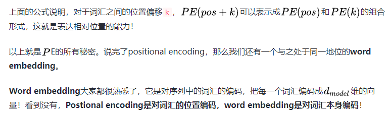
所以，我更喜欢positional encoding的另外一个名字Positional embedding！

Positional encoding的实现

PE的实现也不难，按照论文的公式即可。代码如下：

复制代码import torch
import torch.nn as nnclass PositionalEncoding(nn.Module):def __init__(self, d_model, max_seq_len):"""初始化。Args:d_model: 一个标量。模型的维度，论文默认是512max_seq_len: 一个标量。文本序列的最大长度"""super(PositionalEncoding, self).__init__()# 根据论文给的公式，构造出PE矩阵position_encoding = np.array([[pos / np.pow(10000, 2.0 * (j // 2) / d_model) for j in range(d_model)]for pos in range(max_seq_len)])# 偶数列使用sin，奇数列使用cosposition_encoding[:, 0::2] = np.sin(position_encoding[:, 0::2])position_encoding[:, 1::2] = np.cos(position_encoding[:, 1::2])# 在PE矩阵的第一行，加上一行全是0的向量，代表这`PAD`的positional encoding# 在word embedding中也经常会加上`UNK`，代表位置单词的word embedding，两者十分类似# 那么为什么需要这个额外的PAD的编码呢？很简单，因为文本序列的长度不一，我们需要对齐，# 短的序列我们使用0在结尾补全，我们也需要这些补全位置的编码，也就是`PAD`对应的位置编码pad_row = torch.zeros([1, d_model])position_encoding = torch.cat((pad_row, position_encoding))# 嵌入操作，+1是因为增加了`PAD`这个补全位置的编码，# Word embedding中如果词典增加`UNK`，我们也需要+1。看吧，两者十分相似self.position_encoding = nn.Embedding(max_seq_len + 1, d_model)self.position_encoding.weight = nn.Parameter(position_encoding,requires_grad=False)def forward(self, input_len):"""神经网络的前向传播。Args:input_len: 一个张量，形状为[BATCH_SIZE, 1]。每一个张量的值代表这一批文本序列中对应的长度。Returns:返回这一批序列的位置编码，进行了对齐。"""# 找出这一批序列的最大长度max_len = torch.max(input_len)tensor = torch.cuda.LongTensor if input_len.is_cuda else torch.LongTensor# 对每一个序列的位置进行对齐，在原序列位置的后面补上0# 这里range从1开始也是因为要避开PAD(0)的位置input_pos = tensor([list(range(1, len + 1)) + [0] * (max_len - len) for len in input_len])return self.position_encoding(input_pos)

Word embedding的实现

Word embedding应该是老生常谈了，它实际上就是一个二维浮点矩阵，里面的权重是可训练参数，我们只需要把这个矩阵构建出来就完成了word embedding的工作。

所以，具体的实现很简单：

复制代码import torch.nn as nnembedding = nn.Embedding(vocab_size, embedding_size, padding_idx=0)
# 获得输入的词嵌入编码
seq_embedding = seq_embedding(inputs)*np.sqrt(d_model)

上面vocab_size就是词典的大小，embedding_size就是词嵌入的维度大小，论文里面就是等于
。所以word embedding矩阵就是一个vocab_size*embedding_size的二维张量。

Position-wise Feed-Forward network是什么？

这就是一个全连接网络，包含两个线性变换和一个非线性函数（实际上就是ReLU）。公式如下：

这个线性变换在不同的位置都表现地一样，并且在不同的层之间使用不同的参数。

论文提到，这个公式还可以用两个核大小为1的一维卷积来解释，卷积的输入输出都是
，中间层的维度是。
实现如下：

复制代码import torch
import torch.nn as nnclass PositionalWiseFeedForward(nn.Module):def __init__(self, model_dim=512, ffn_dim=2048, dropout=0.0):super(PositionalWiseFeedForward, self).__init__()self.w1 = nn.Conv1d(model_dim, ffn_dim, 1)self.w2 = nn.Conv1d(model_dim, ffn_dim, 1)self.dropout = nn.Dropout(dropout)self.layer_norm = nn.LayerNorm(model_dim)def forward(self, x):output = x.transpose(1, 2)output = self.w2(F.relu(self.w1(output)))output = self.dropout(output.transpose(1, 2))# add residual and norm layeroutput = self.layer_norm(x + output)return output

Transformer的实现

至此，所有的细节都已经解释完了。现在来完成我们Transformer模型的代码。

首先，我们需要实现6层的encoder和decoder。

encoder代码实现如下：

复制代码import torch
import torch.nn as nnclass EncoderLayer(nn.Module):"""Encoder的一层。"""def __init__(self, model_dim=512, num_heads=8, ffn_dim=2018, dropout=0.0):super(EncoderLayer, self).__init__()self.attention = MultiHeadAttention(model_dim, num_heads, dropout)self.feed_forward = PositionalWiseFeedForward(model_dim, ffn_dim, dropout)def forward(self, inputs, attn_mask=None):# self attentioncontext, attention = self.attention(inputs, inputs, inputs, padding_mask)# feed forward networkoutput = self.feed_forward(context)return output, attentionclass Encoder(nn.Module):"""多层EncoderLayer组成Encoder。"""def __init__(self,vocab_size,max_seq_len,num_layers=6,model_dim=512,num_heads=8,ffn_dim=2048,dropout=0.0):super(Encoder, self).__init__()self.encoder_layers = nn.ModuleList([EncoderLayer(model_dim, num_heads, ffn_dim, dropout) for _ inrange(num_layers)])self.seq_embedding = nn.Embedding(vocab_size + 1, model_dim, padding_idx=0)self.pos_embedding = PositionalEncoding(model_dim, max_seq_len)def forward(self, inputs, inputs_len):output = self.seq_embedding(inputs)output += self.pos_embedding(inputs_len)self_attention_mask = padding_mask(inputs, inputs)attentions = []for encoder in self.encoder_layers:output, attention = encoder(output, self_attention_mask)attentions.append(attention)return output, attentions

通过文章前面的分析，代码不需要更多解释了。同样的，我们的decoder代码如下：

复制代码import torch
import torch.nn as nnclass DecoderLayer(nn.Module):def __init__(self, model_dim, num_heads=8, ffn_dim=2048, dropout=0.0):super(DecoderLayer, self).__init__()self.attention = MultiHeadAttention(model_dim, num_heads, dropout)self.feed_forward = PositionalWiseFeedForward(model_dim, ffn_dim, dropout)def forward(self,dec_inputs,enc_outputs,self_attn_mask=None,context_attn_mask=None):# self attention, all inputs are decoder inputsdec_output, self_attention = self.attention(dec_inputs, dec_inputs, dec_inputs, self_attn_mask)# context attention# query is decoder's outputs, key and value are encoder's inputsdec_output, context_attention = self.attention(enc_outputs, enc_outputs, dec_output, context_attn_mask)# decoder's output, or contextdec_output = self.feed_forward(dec_output)return dec_output, self_attention, context_attentionclass Decoder(nn.Module):def __init__(self,vocab_size,max_seq_len,num_layers=6,model_dim=512,num_heads=8,ffn_dim=2048,dropout=0.0):super(Decoder, self).__init__()self.num_layers = num_layersself.decoder_layers = nn.ModuleList([DecoderLayer(model_dim, num_heads, ffn_dim, dropout) for _ inrange(num_layers)])self.seq_embedding = nn.Embedding(vocab_size + 1, model_dim, padding_idx=0)self.pos_embedding = PositionalEncoding(model_dim, max_seq_len)def forward(self, inputs, inputs_len, enc_output, context_attn_mask=None):output = self.seq_embedding(inputs)output += self.pos_embedding(inputs_len)self_attention_padding_mask = padding_mask(inputs, inputs)seq_mask = sequence_mask(inputs)self_attn_mask = torch.gt((self_attention_padding_mask + seq_mask), 0)self_attentions = []context_attentions = []for decoder in self.decoder_layers:output, self_attn, context_attn = decoder(output, enc_output, self_attn_mask, context_attn_mask)self_attentions.append(self_attn)context_attentions.append(context_attn)return output, self_attentions, context_attentions

最后，我们把encoder和decoder组成Transformer模型！

代码如下：

复制代码import torch
import torch.nn as nnclass Transformer(nn.Module):def __init__(self,src_vocab_size,src_max_len,tgt_vocab_size,tgt_max_len,num_layers=6,model_dim=512,num_heads=8,ffn_dim=2048,dropout=0.2):super(Transformer, self).__init__()self.encoder = Encoder(src_vocab_size, src_max_len, num_layers, model_dim,num_heads, ffn_dim, dropout)self.decoder = Decoder(tgt_vocab_size, tgt_max_len, num_layers, model_dim,num_heads, ffn_dim, dropout)self.linear = nn.Linear(model_dim, tgt_vocab_size, bias=False)self.softmax = nn.Softmax(dim=2)def forward(self, src_seq, src_len, tgt_seq, tgt_len):context_attn_mask = padding_mask(tgt_seq, src_seq)output, enc_self_attn = self.encoder(src_seq, src_len)output, dec_self_attn, ctx_attn = self.decoder(tgt_seq, tgt_len, output, context_attn_mask)output = self.linear(output)output = self.softmax(output)return output, enc_self_attn, dec_self_attn, ctx_attn

至此，Transformer模型已经实现了！

如何学习大模型 AI ？

由于新岗位的生产效率，要优于被取代岗位的生产效率，所以实际上整个社会的生产效率是提升的。

但是具体到个人，只能说是：

“最先掌握AI的人，将会比较晚掌握AI的人有竞争优势”。

这句话，放在计算机、互联网、移动互联网的开局时期，都是一样的道理。

我在一线互联网企业工作十余年里，指导过不少同行后辈。帮助很多人得到了学习和成长。

我意识到有很多经验和知识值得分享给大家，也可以通过我们的能力和经验解答大家在人工智能学习中的很多困惑，所以在工作繁忙的情况下还是坚持各种整理和分享。但苦于知识传播途径有限，很多互联网行业朋友无法获得正确的资料得到学习提升，故此将并将重要的AI大模型资料包括AI大模型入门学习思维导图、精品AI大模型学习书籍手册、视频教程、实战学习等录播视频免费分享出来。

第一阶段（10天）：初阶应用

该阶段让大家对大模型 AI有一个最前沿的认识，对大模型 AI 的理解超过 95% 的人，可以在相关讨论时发表高级、不跟风、又接地气的见解，别人只会和 AI 聊天，而你能调教 AI，并能用代码将大模型和业务衔接。

• 大模型 AI 能干什么？
• 大模型是怎样获得「智能」的？
• 用好 AI 的核心心法
• 大模型应用业务架构
• 大模型应用技术架构
• 代码示例：向 GPT-3.5 灌入新知识
• 提示工程的意义和核心思想
• Prompt 典型构成
• 指令调优方法论
• 思维链和思维树
• Prompt 攻击和防范
• …

第二阶段（30天）：高阶应用

该阶段我们正式进入大模型 AI 进阶实战学习，学会构造私有知识库，扩展 AI 的能力。快速开发一个完整的基于 agent 对话机器人。掌握功能最强的大模型开发框架，抓住最新的技术进展，适合 Python 和 JavaScript 程序员。

• 为什么要做 RAG
• 搭建一个简单的 ChatPDF
• 检索的基础概念
• 什么是向量表示（Embeddings）
• 向量数据库与向量检索
• 基于向量检索的 RAG
• 搭建 RAG 系统的扩展知识
• 混合检索与 RAG-Fusion 简介
• 向量模型本地部署
• …

第三阶段（30天）：模型训练

恭喜你，如果学到这里，你基本可以找到一份大模型 AI相关的工作，自己也能训练 GPT 了！通过微调，训练自己的垂直大模型，能独立训练开源多模态大模型，掌握更多技术方案。

到此为止，大概2个月的时间。你已经成为了一名“AI小子”。那么你还想往下探索吗？

• 为什么要做 RAG
• 什么是模型
• 什么是模型训练
• 求解器 & 损失函数简介
• 小实验2：手写一个简单的神经网络并训练它
• 什么是训练/预训练/微调/轻量化微调
• Transformer结构简介
• 轻量化微调
• 实验数据集的构建
• …

第四阶段（20天）：商业闭环

对全球大模型从性能、吞吐量、成本等方面有一定的认知，可以在云端和本地等多种环境下部署大模型，找到适合自己的项目/创业方向，做一名被 AI 武装的产品经理。

• 硬件选型
• 带你了解全球大模型
• 使用国产大模型服务
• 搭建 OpenAI 代理
• 热身：基于阿里云 PAI 部署 Stable Diffusion
• 在本地计算机运行大模型
• 大模型的私有化部署
• 基于 vLLM 部署大模型
• 案例：如何优雅地在阿里云私有部署开源大模型
• 部署一套开源 LLM 项目
• 内容安全
• 互联网信息服务算法备案
• …

学习是一个过程，只要学习就会有挑战。天道酬勤，你越努力，就会成为越优秀的自己。

如果你能在15天内完成所有的任务，那你堪称天才。然而，如果你能完成 60-70% 的内容，你就已经开始具备成为一名大模型 AI 的正确特征了。

这份完整版的大模型 AI 学习资料已经上传CSDN，朋友们如果需要可以微信扫描下方CSDN官方认证二维码免费领取【保证100%免费】