作业用到的知识:
1.Pytorch:
1. nn.Conv2d(二维卷积层)
作用:
对输入的多通道二位数据(如图像)进行特征提取,通过滑动卷积核计算局部区域的加权和,生成新的特征图。
关键参数:
| 参数 | 类型 | 说明 | |
| in_channel | int | 输入的通道NCHW中的C | 3(RGB图像的通道) |
| out_channels | int | 输出的通道数(卷积核数量) | 64(生成64个特征图) |
| kernel size | int/tuple | 卷积核尺寸 | 3(3X3)或(3,5) |
| stride | int/tuple | 卷积核滑动步长 | 2 |
| padding | int/tuple | 输入边缘填充像素数 | |
| dilation | int/tuple | 卷积核元素间距(扩张卷积) | 2 |
| groups | int | 分组卷积的数组 | groups= in_channels(深度可分离卷积) |
| bias | bool | 是否添加偏置项 | False(配合Batch Norm时使用) |
输入输出形状
-
输入:
(N, C_in, H_in, W_in) -
输出:
(N, C_out, H_out, W_out) -
-
2. nn.BatchNorm2d
作用:
对每个通道的特征图进行归一化(均值归零、方差归一),加速训练、缓解梯度消失/爆炸,并允许使用更大的学习率
| 参数 | 类型 | 说明 | 示例 |
| num_feature | int | C | 64 |
| eps | float | 数值稳定性系数(防止除以0) | 1e-5 |
| momentum | float | 更新运行均值/方差的动量系数 | 0.1 |
| affine | bool | 是否学习缩放因子 | True(默认启用 |
-
输入:
(N, C, H, W) -
输出:
(N, C, H, W)(形状不变) -
归一化公式:
-
对每个通道独立计算:
-
-
3 nn.ReLU(True)(修正线性单元激活函数)
作用
-
激活函数:引入非线性,使神经网络能够学习复杂的模式。
-
数学公式:
ReLU(x)=max(0,x)-
输入为负时输出0,输入为正时保持不变。
-
参数 inplace=True
-
功能:直接在输入张量上进行修改(覆盖原数据),节省内存。
-
为什么用ReLU?
-
稀疏性:负值归零,使网络更稀疏,提升计算效率。
-
缓解梯度消失:正区间的梯度恒为1,避免深层网络梯度消失问题。
4. nn.MaxPool2d(2, 2)(二维最大池化层)
作用
-
下采样:降低特征图的空间尺寸(高度和宽度),减少计算量。
-
保留显著特征:取局部区域的最大值,保留最显著的特征。
参数解析
-
kernel_size=2:池化窗口大小为2×2。 -
stride=2:窗口每次移动2步(水平和垂直方向)。 -
默认行为:
-
若未指定
padding,默认不填充(padding=0)。 -
若未指定
dilation,默认窗口连续无间隔。 -
输出尺寸公式:
-
-
为什么用最大池化?
-
平移不变性:对特征的位置变化更鲁棒。
-
降维提速:减少后续层的计算量。
-
5. flatten和linear
| 组件 | 功能 | 关键参数 | 输入输出示例 |
|---|---|---|---|
nn.Flatten() | 将多维数据展平为一维向量 | start_dim, end_dim | [2,3,4,4] → [2,48] |
nn.Linear | 线性变换(分类/回归) (即 | in_features, out_features | [2,48] → [2,10] |
-
nn.Flatten()是连接卷积层和全连接层的桥梁,解决多维数据与一维输入的维度不匹配问题。 -
nn.Linear通过线性变换实现特征到目标的映射,是神经网络的最终决策层。
6.Pytorch初始化方法
| 初始化方法 | 函数 | 适用场景 |
|---|---|---|
| Xavier 正态分布 | xavier_normal_ | tanh/sigmoid 激活 |
| He 正态分布(Kaiming) | kaiming_normal_ | ReLU/LeakyReLU 激活 |
| 均匀分布 | uniform_ | 简单初始化 |
| 常数初始化 | constant_ | 特殊需求(如全零初始化) |
7. BCELoss 损失函数
torch.nn.BCELoss() 是 PyTorch 中用于 二分类任务 的交叉熵损失函数,适用于模型输出为 概率值(即属于正类的概率)的场景:
核心公式与功能
1). 数学公式
对于每个样本,损失计算为:
loss(x,y)=−[y⋅log(x)+(1−y)⋅log(1−x)]
-
x:模型输出的概率值(需在 [0, 1] 范围内)。
-
yy:真实标签(取值为 0 或 1)
2). 功能
-
衡量 模型预测概率 与 真实标签 之间的差距。
-
优化目标:使预测概率尽可能接近真实标签。
3)使用步骤
模型输出处理
确保模型最后一层使用 Sigmoid 激活函数,将输出压缩到 [0, 1] 区间:
model = nn.Sequential(nn.Linear(input_dim, 1),nn.Sigmoid()  # 必须添加 Sigmoid
)
计算损失
criterion = nn.BCELoss()
output = model(x)          # 输出形状 (N, *)
loss = criterion(output, target)
4) 反向传播
调用 loss.backward() 时,PyTorch 的 Autograd 系统自动执行以下操作:
-
计算损失对模型输出的梯度:
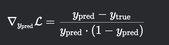
这一步由
BCELoss的反向函数自动实现。 -
梯度反向传播到前一层:
-
如果模型输出 ypredypred 是 Sigmoid 的输出,梯度会继续反向传播到 Sigmoid 的输入 zz(即线性层的输出)。
-
根据链式法则,梯度在 Sigmoid 层被修正为
 。
。
-
-
更新模型参数:
-
梯度从 Sigmoid 层传播到线性层的权重和偏置。
-
优化器(如
optimizer.step())根据梯度更新参数。
-
python:
1.np.random.permutation
np.random.permutation 是 NumPy 中用于生成随机排列的函数。它可以对数组元素进行随机打乱,或生成一个范围序列的随机排列。以下是具体用法和场景:
功能概述
-
输入为整数
n:生成[0, 1, 2, ..., n-1]的随机排列。 -
输入为数组:返回数组元素的随机排列(不修改原数组)。
-
与
np.random.shuffle的区别:shuffle直接修改原数组,而permutation返回新数组,原数组不变。
1). 生成整数序列的随机排列
import numpy as np# 生成 0-4 的随机排列
arr = np.random.permutation(5)
print(arr)  # 输出示例:[3 1 4 0 2]
2). 打乱数组元素的顺序
original = np.array([10, 20, 30, 40, 50])
shuffled = np.random.permutation(original)
print("原数组:", original)  # 原数组: [10 20 30 40 50]
print("打乱后:", shuffled)   # 打乱后: [30 10 50 40 20]
2. os.path.join
os.path.join(data_path, 'cats')作用:将
data_path(基础路径)与子目录cats拼接成完整路径。
os.listdir(os.path.join(data_path, 'cats'))作用:获取
cats目录下的所有条目(文件和子目录)名称列表。
sorted(...)
作用:对
os.listdir返回的列表按字母顺序升序排列。
执行结果:
cat_dirs:排序后的cats目录内容列表,如['cat1.jpg', 'cat2.jpg', 'subfolder']。
dog_dirs:排序后的dogs目录内容列表,如['dog1.jpg', 'dog2.jpg']。
3.np.expand_dims 的作用
-
功能:在指定轴(
axis)插入一个新维度,扩展数组的形状。 -
语法:
python
复制
np.expand_dims(arr, axis)
Pytorch实现基本的CNN和实验结果
1. 获取数据集:
import kagglehub
import shutil# Download latest version
path = kagglehub.dataset_download("fusicfenta/cat-and-dog")# 自定义目标路径
custom_path = "/Users/hailie/Desktop/小兰/hailie/study/AI/DL/coursera作业/DL_homework_self/CNN/"# 将文件移动到自定义路径
shutil.move(path, custom_path)print("数据集已移动到:", custom_path)
import os
from typing import Tuple
import cv2
import numpy as npdef load_set(data_path: str, cnt: int, img_shape: Tuple[int,int]):cat_dirs = sorted(os.listdir(os.path.join(data_path, 'cats')))dog_dirs = sorted(os.listdir(os.path.join(data_path, 'dogs')))images = []for i, cat_dir in enumerate(cat_dirs):if i >= cnt:breakname = os.path.join(data_path, 'cats', cat_dir)cat = cv2.imread(name)images.append(cat)for i, dog_dir in enumerate(dog_dirs):if i >= cnt:breakname = os.path.join(data_path, 'dogs', dog_dir)dog = cv2.imread(name)images.append(dog)for i in range(len(images)):images[i] = cv2.resize(images[i],img_shape)images[i] = images[i].astype(np.float32) /255.0return np.array(images) def get_cat_set(data_path: str,img_shape: Tuple[int, int] = (224, 224),train_size = 1000,test_size = 200)->Tuple[np.ndarray, np.ndarray, np.ndarray, np. ndarray]:train_X = load_set(os.path.join(data_path,'training_set'),train_size,img_shape)test_X= load_set(os.path.join(data_path,'test_set'),test_size,img_shape)train_Y = np.array([1]* train_size + [0] * train_size)test_Y = np.array([1] * test_size + [0] * test_size)train_X = np.reshape(train_X,(-1,3,*img_shape))test_X = np.reshape(test_X,(-1,3,*img_shape))return train_X, np.expand_dims(train_Y,1), test_X, np.expand_dims(test_Y,1)
train_X = np.reshape(train_X, (-1, 3, *img_shape)
test_X = np.reshape(test_X, (-1, 3, *img_shape)
-
输入数据
train_X/test_X:通过reshape调整形状为NCHW格式。-
-1:自动推断批次数N(保持总数据量不变)。 -
3:通道数(例如 RGB 图像的通道数)。 -
*img_shape:展开图像的高度和宽度(例如img_shape = (32, 32)→32, 32)。 -
示例:
原始形状为(N, H, W, 3)(NHWC) → 调整后为(N, 3, H, W)(NCHW)
-
2. 初始化模型:
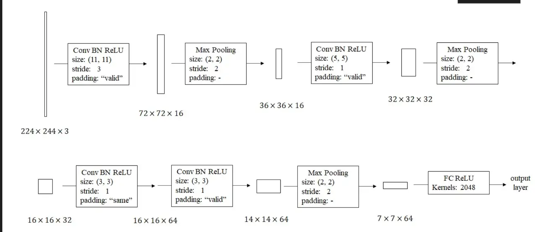
由于这个二分类任务比较简单,我在设计时尽可能让可训练参数更少。刚开始用一个大步幅、大卷积核的卷积快速缩小图片边长,之后逐步让图片边长减半、深度翻倍。
这样一个网络用PyTorch实现如下:
import torch
import numpy as np
import torch.nn as nn
import mathdef init_model():model = nn.Sequential(nn.Conv2d(3,16,11,3),nn.BatchNorm2d(16),nn.ReLU(True), nn.MaxPool2d(2,2),nn.Conv2d(16,32,5),nn.BatchNorm2d(32),nn.ReLU(True),nn.MaxPool2d(2,2),nn.Conv2d(32,64,3,padding=1),nn.BatchNorm2d(64),nn.ReLU(True),nn.Conv2d(64,64,3),nn.BatchNorm2d(64),nn.ReLU(True),nn.MaxPool2d(2,2),nn.Flatten(),nn.Linear(3136,2048), nn.ReLU(True),nn.Linear(2048,1),nn.Sigmoid())def weights_init(m):if isinstance(m,nn.Conv2d):torch.nn.init.xavier_normal_(m.weight)m.bias.data.fill_(0)elif isinstance(m,nn.BatchNorm2d):m.weight.data.normal_(1.0,0.02) # 默认简单初始化m.bias.data.fill_(0)elif isinstance(m,nn.Linear):torch.nn.init.xavier_normal_(m.weight)m.bias.data.fill_(0)model.apply(weights_init)print(model)return modeltorch.nn.Sequential()用于创建一个串行的网络(前一个模块的输出就是后一个模块的输入)。网络各模块用到的初始化参数的介绍如下:
Conv2d: 输入通道数、输出通道数、卷积核边长、步幅、填充个数padding。BatchNormalization: 输入通道数。ReLU: 一个bool值inplace。是否使用inplace,就和用a += 1还是a + 1一样,后者会多花一个中间变量来存结果。MaxPool2d: 卷积核边长、步幅。Linear(全连接层):输入通道数、输出通道数。
根据之前的设计,把参数填入这些模块即可。
由于PyTorch在初始化模块时不能自动初始化参数,我们要手动写上初始化参数的逻辑。
在此之前,要先认识一下torch.nn.Module的apply函数。
model.apply(weights_init)PyTorch的模型模块torch.nn.Module是自我嵌套的。一个torch.nn.Module的实例可能由多个torch.nn.Module的实例组成。model.apply(func)可以对某torch.nn.Module实例的所有某子模块执行func函数。我们使用的参数初始化函数叫做weights_init,所以用上面那行代码就可以初始化所有模块。
其中,m就是子模块的示例。通过对其进行类型判断,我们可以对不同的模块执行不同的初始化方式。初始化的函数都在torch.nn.init,这里用的是torch.nn.init.xavier_normal_。
3. 准备优化器和loss
初始化完模型后,可以用下面的代码初始化优化器与loss。
model = init_model(device)
optimizer = torch.optim.Adam(model.parameters(), 5e-4)
loss_fn = torch.nn.BCELoss()
torch.optim.Adam可以初始化一个Adam优化器。它的第一个参数是所有可训练参数,直接对一个torch.nn.Module调用.parameters()即可一键获取参数。它的第二个参数是学习率,这个可以根据实验情况自行调整。
torch.nn.BCELoss是二分类用到的交叉熵误差。这里只是对它进行了初始化。在调用时,使用方法是loss(input, target)。input是用于比较的结果,target是被比较的标签。
4.训练与推理
def train(model:nn.Module,train_X:np.ndarray,train_Y:np.ndarray,optimizer:torch.optim.Optimizer,loss_fn:nn.Module,batch_size:int,num_epoch: int):m = train_X.shape[0]#print("m:",m,"batch_size,",batch_size)print(train_X.shape) # (m, 3, 224, 224)print(train_Y.shape) # (m, 1)indices = np.random.permutation(m)num_mini_batch = math.ceil(m / batch_size)mini_batch_XYs = []shuffle_X = train_X[indices, ...]shuffle_Y = train_Y[indices, ...]for i in range(num_mini_batch):if i == num_mini_batch - 1:mini_batch_X = shuffle_X[i*batch_size:,...]mini_batch_Y = shuffle_Y[i*batch_size:,...]else:mini_batch_X = shuffle_X[i*batch_size: (i+1)*batch_size, ...]mini_batch_Y = shuffle_Y[i*batch_size: (i+1)*batch_size, ...]mini_batch_X = torch.from_numpy(mini_batch_X)mini_batch_Y = torch.from_numpy(mini_batch_Y).float()mini_batch_XYs.append((mini_batch_X,mini_batch_Y))print(f'Num mini-batch:{num_mini_batch}')for e in range(num_epoch):for mini_batch_X, mini_batch_Y in mini_batch_XYs:mini_batch_Y_hat = model(mini_batch_X)loss: torch.Tensor = loss_fn(mini_batch_Y_hat, mini_batch_Y)optimizer.zero_grad()loss.backward()optimizer.step()print(f'Epoch{e}. loss:{loss}')def evaluate (model: nn.Module,test_X:np.ndarray,test_Y: np.ndarray):test_X = torch.from_numpy(test_X)test_Y = torch.from_numpy(test_Y)test_Y_hat = model(test_X)predicts = torch.where(test_Y_hat>0.5,1,0)score = torch.where(predicts == test_Y, 1.0, 0.0)acc = torch.mean(score)print(f'Accuracy: {acc}')
在训练时,我们采用mini-batch策略。因此,开始迭代前,我们要编写预处理mini-batch的代码
这里还有一些有关PyTorch的知识需要讲解。torch.from_numpy可以把一个NumPy数组转换成torch.Tensor。由于标签Y是个整形张量,而PyTorch算loss时又要求标签是个float,这里要调用.float()把张量强制类型转换到float型。同理,其他类型也可以用类似的方法进行转换。
直接用model(x)即可让模型model执行输入x的前向传播。
之后几行代码就属于训练的常规操作了。先计算loss,再清空优化器的梯度,做反向传播,最后调用优化器更新所有参数。
train_X, train_Y, test_X, test_Y = get_cat_set('/Users/hailie/Desktop/小兰/hailie/study/AI/DL/coursera作业/DL_homework_self/CNN/1/dataset',train_size=1000)cnn_model = init_model()
optimizer = torch.optim.Adam(cnn_model.parameters(), 5e-4)
loss_fn = torch.nn.BCELoss()
train(cnn_model, train_X,train_Y, optimizer, loss_fn, 16, 5)
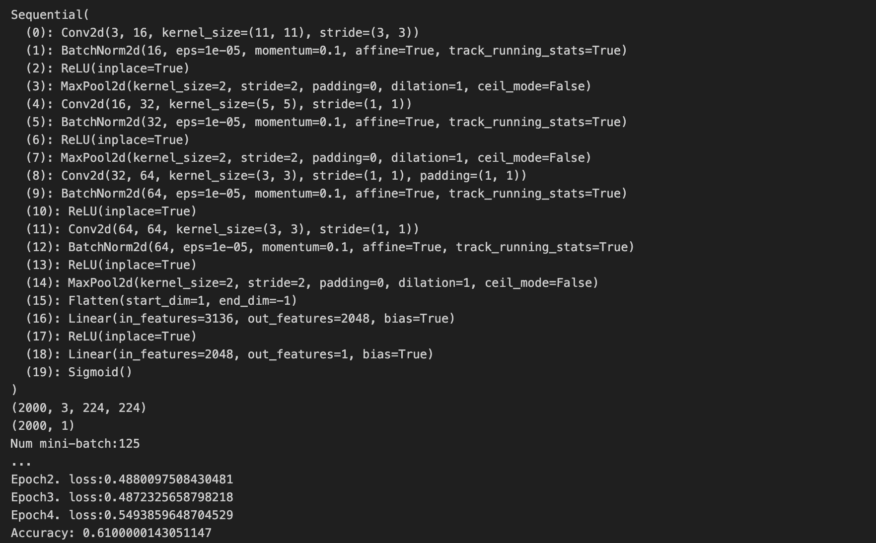
evaluate(cnn_model, test_X, test_Y)5.实验结果
电脑资源受限,只跑了一点点
用Numpy复现一致的torch.conv2d
为了加深理解 下面用NumPy复现一致的torch.conv2d向前传播
再回顾一下主要参数:
主要参数
-
in_channels (int)
-
作用:输入数据的通道数(例如,RGB 图像为 3,灰度图为 1)。
-
示例:
in_channels=3
-
-
out_channels (int)
-
作用:输出特征图的通道数(即卷积核的数量)。
-
示例:
out_channels=64表示生成 64 个特征图。
-
-
kernel_size (int 或 tuple)
-
作用:卷积核的尺寸。可以是单个整数(如
3表示 3×3)或元组(如(3,5))。 -
示例:
kernel_size=3或kernel_size=(3,5)
-
-
stride (int 或 tuple, 默认
1)-
作用:卷积核的步长。控制输出尺寸的缩小比例。
-
示例:
stride=2或stride=(2,1)
-
-
padding (int 或 tuple, 默认
0)-
作用:输入数据的边缘填充像素数。用于控制输出尺寸。
-
示例:
padding=1表示在四周各填充 1 行/列。
-
-
dilation (int 或 tuple, 默认
1)-
作用:卷积核元素的间距(扩张卷积)。增大感受野,不增加参数量。
-
示例:
dilation=2时,3×3 卷积核的感受野等效于 5×5。 -
-
-
groups (int, 默认
1)-
作用:分组卷积的组数。
groups=in_channels时为深度可分离卷积。 -
约束:
in_channels和out_channels必须能被groups整除。 -
示例:
groups=2表示将输入和输出的通道分为 2 组独立卷积。 -
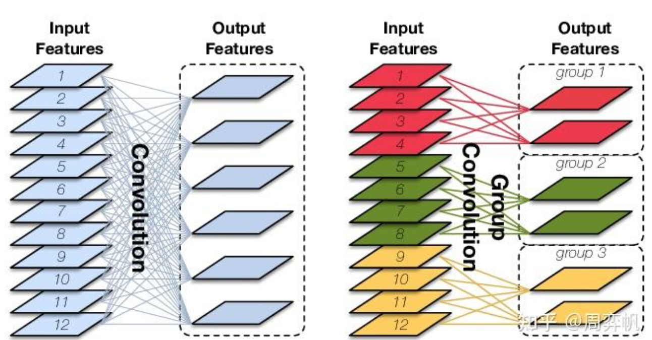
下图展示了输入通道数12,输出通道数6的卷积在两种不同groups下的情况。左边是group=1的普通卷积,右边是groups=3的分组卷积。在具体看分组卷积的介绍前,
-
-
-
bias (bool, 默认
True)-
作用:是否添加偏置项。若后续接 BatchNorm 层,通常设为
False。 -
示例:
bias=False
-
向前传播
import numpy as np
import pytest
import torchdef conv2d(input: np.ndarray,weight: np.ndarray,stride: int,padding: int,dilation: int,groups: int,bias:np.ndarray = None)->np.ndarray:#Args:#input (np.ndarray): The input NumPy array of shape (H, W, C).#weight (np.ndarray): The weight NumPy array of shape#    (C', F, F, C / groups).#stride (int): Stride for convolution.#padding (int): The count of zeros to pad on both sides.#dilation (int): The space between kernel elements.#groups (int): Split the input to groups.#bias (np.ndarray | None): The bias NumPy array of shape (C').h_input, w_input, c_input = input.shapec_o, f, f_2, c_k = weight.shapeassert(f==f_2)assert(c_input % groups == 0)assert(c_o % groups ==0)assert(c_input // groups == c_k)if bias is not None:assert(bias.shape[0] == c_o)f_new = f + (f-1) * (dilation -1)weight_new = np.zeros((c_o, f_new, f_new, c_k), dtype=weight.dtype)for i_c_o in range(c_o):for i_c_k in range(c_k):for i_f in range(f):for j_f in range(f):i_f_new = i_f * dilationj_f_new = j_f * dilation          weight_new [i_c_o, i_f_new, j_f_new, i_c_k] = weight[i_c_o,i_f,j_f,i_c_k]input_pad = np.pad(input, [(padding, padding),(padding, padding),(0,0)])def cal_new_sidelength(size, stride,f, padding):return ((size + 2*padding - f) // stride) +1h_output = cal_new_sidelength(h_input, stride, f_new, padding)w_output = cal_new_sidelength(w_input, stride, f_new, padding)output = np.empty((h_output, w_output,c_o), dtype=input.dtype)c_o_per_group = c_o // groupsfor i_h in range(h_output):for i_w in range(w_output):for i_c in range(c_o):i_g = i_c//c_o_per_groupvert_start = i_h * stridevert_end = vert_start + f_newhoriz_start = i_w * stridehoriz_end = horiz_start + f_newchannel_start = c_k * i_gchannel_end = c_k * (i_g + 1)input_slice = input_pad[vert_start : vert_end,horiz_start:horiz_end,channel_start:channel_end]kernel_slice = weight_new[i_c]output[i_h,i_w,i_c] = np.sum(input_slice * kernel_slice)if bias:output[i_h,i_w,i_c] += bias[i_c]return output@pytest.mark.parametrize('c_i, c_o', [(3, 6), (2, 2)])
@pytest.mark.parametrize('kernel_size', [3, 5])
@pytest.mark.parametrize('stride', [1, 2])
@pytest.mark.parametrize('padding', [0, 1])
@pytest.mark.parametrize('dilation', [1, 2])
@pytest.mark.parametrize('groups', ['1', 'all'])
@pytest.mark.parametrize('bias', [False])
def test_conv(c_i: int, c_o: int, kernel_size: int, stride: int, padding: str,dilation: int, groups: str, bias: bool):if groups == '1':groups = 1elif groups == 'all':groups = c_iif bias:bias = np.random.randn(c_o)torch_bias = torch.from_numpy(bias)else:bias = Nonetorch_bias = Noneinput = np.random.randn(20, 20, c_i)weight = np.random.randn(c_o, kernel_size, kernel_size, c_i // groups)torch_input = torch.from_numpy(np.transpose(input, (2, 0, 1))).unsqueeze(0)torch_weight = torch.from_numpy(np.transpose(weight, (0, 3, 1, 2)))torch_output = torch.conv2d(torch_input, torch_weight, torch_bias, stride,padding, dilation, groups).numpy()torch_output = np.transpose(torch_output.squeeze(0), (1, 2, 0))numpy_output = conv2d(input, weight, stride, padding, dilation, groups,bias)assert np.allclose(torch_output, numpy_output)
input的形状是(H,W,C)卷积核组weight形状是(C',H,W,C_k), 其中C_k = C/groups。同时 C'也必须能够被groups整除。bias形状是C'。
空洞卷积可以用卷积核扩充实现。因此,在开始卷积之前,可以先预处理好扩充后的卷积核。我们先算好扩充后卷积核的形状,并创建好新的卷积核,最后用多重循环给新卷积核赋值。
f_new = f + (f - 1) * (dilation - 1)weight_new = np.zeros((c_o, f_new, f_new, c_k), dtype=weight.dtype)for i_c_o in range(c_o):for i_c_k in range(c_k):for i_f in range(f):for j_f in range(f):i_f_new = i_f * dilationj_f_new = j_f * dilationweight_new[i_c_o, i_f_new, j_f_new, i_c_k] = \weight[i_c_o, i_f, j_f, i_c_k]
@pytest.mark.parametrize用于设置单元测试参数的可选值。我设置了6组参数,每组参数有2个可选值,经过排列组合后可以生成2^6=64个单元测试,pytest会自动帮我们执行不同的测试。
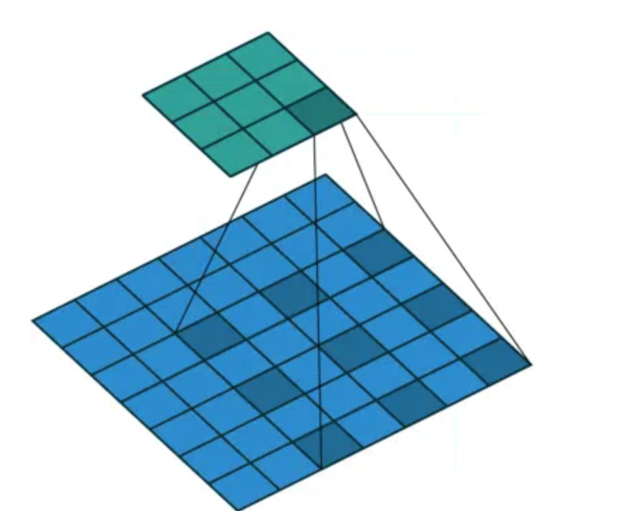
向后传播
向前传播时,我们遍历输出图像的每一个位置,选择该位置对应的输入图像切片和卷积核,做一遍乘法,再加上bias。
其实,一轮运算写成数学公式的话,就是一个线性函数y=wx+b。对w, x, b求导非常简单:
dw_i = x * dy
dx_i = w * dy
db_i = dy
在反向传播中,我们只需要遍历所有这样的线性运算,计算这轮运算对各参数的导数的贡献即可。最后,累加所有的贡献,就能得到各参数的导数。当然,在用代码实现这段逻辑时,可以不用最后再把所有贡献加起来,而是一算出来就加上。
dw += x * dy
dx += w * dy
db += dy这里要稍微补充一点。在前向传播的实现中,我加入了dilation, groups这两个参数。为了简化反向传播的实现代码,只展示反向传播中最精华的部分,我在这份卷积实现中没有使用这两个参数。
from typing import Dict, Tupleimport numpy as np
import pytest
import torchdef conv2d_forward(input: np.ndarray, weight: np.ndarray, bias: np.ndarray,stride: int, padding: int) -> Dict[str, np.ndarray]:"""2D Convolution Forward Implemented with NumPy.Args:input (np.ndarray): The input NumPy array of shape (H, W, C).weight (np.ndarray): The weight NumPy array of shape(C', F, F, C).bias (np.ndarray | None): The bias NumPy array of shape (C').Default: None.stride (int): Stride for convolution.padding (int): The count of zeros to pad on both sides.Outputs:Dict[str, np.ndarray]: Cached data for backward prop."""h_i, w_i, c_i = input.shapec_o, f, f_2, c_k = weight.shapeassert (f == f_2)assert (c_i == c_k)assert (bias.shape[0] == c_o)input_pad = np.pad(input, [(padding, padding), (padding, padding), (0, 0)])def cal_new_sidelngth(sl, s, f, p):return (sl + 2 * p - f) // s + 1h_o = cal_new_sidelngth(h_i, stride, f, padding)w_o = cal_new_sidelngth(w_i, stride, f, padding)output = np.empty((h_o, w_o, c_o), dtype=input.dtype)for i_h in range(h_o):for i_w in range(w_o):for i_c in range(c_o):h_lower = i_h * strideh_upper = i_h * stride + fw_lower = i_w * stridew_upper = i_w * stride + finput_slice = input_pad[h_lower:h_upper, w_lower:w_upper, :]kernel_slice = weight[i_c]output[i_h, i_w, i_c] = np.sum(input_slice * kernel_slice)output[i_h, i_w, i_c] += bias[i_c]cache = dict()cache['Z'] = outputcache['W'] = weightcache['b'] = biascache['A_prev'] = inputreturn cachedef conv2d_backward(dZ:np.ndarray,cache:dict[str:np.ndarray],stride:int,padding:int)->Tuple[np.ndarray,np.ndarray,np.ndarray]:Z = cache['Z']W = cache['W']b = cache['b']A_prev = cache['A_prev']dW = np.zeros(W.shape)db = np.zeros(b.shape)dA_prev = np.zeros(A_prev.shape)A_prev_pad = np.pad(A_prev, [(padding,padding),(padding,padding),(0,0)])dA_prev_pad = np.pad(dA_prev, [(padding,padding),(padding,padding),(0,0)])h_o,w_o,c_o_2 = dZ.shapec_o,f,f_2,c_k = W.shape_,_,c_i = A_prev.shapeassert (f == f_2)assert (c_i == c_k)assert (c_o == c_o_2)for i_h in range(h_o):for i_w in range(w_o):for i_c in range(c_o):vert_start = i_h * stridehoriz_start = i_w * stridevert_end = vert_start + fhoriz_end = horiz_start + finput_slice = A_prev_pad[vert_start:vert_end,horiz_start:horiz_end,:]dW[i_c] += input_slice * dZ[i_h,i_w,i_c]dA_prev_pad[vert_start:vert_end, horiz_start:horiz_end,:] +=W[i_c] *dZ[i_h,i_w,i_c]db[i_c] += dZ[i_h,i_w,i_c]if padding > 0:dA_prev = dA_prev_pad[padding:-padding, padding:-padding, :]else:dA_prev = dA_prev_padreturn dW, db, dA_prev@pytest.mark.parametrize('c_i, c_o', [(3, 6), (2, 2)])
@pytest.mark.parametrize('kernel_size', [3, 5])
@pytest.mark.parametrize('stride', [1, 2])
@pytest.mark.parametrize('padding', [0, 1])
def test_conv(c_i: int, c_o: int, kernel_size: int, stride: int, padding: str):# Preprocessinput = np.random.randn(20, 20, c_i)weight = np.random.randn(c_o, kernel_size, kernel_size, c_i)bias = np.random.randn(c_o)torch_input = torch.from_numpy(np.transpose(input, (2, 0, 1))).unsqueeze(0).requires_grad_()torch_weight = torch.from_numpy(np.transpose(weight, (0, 3, 1, 2))).requires_grad_()torch_bias = torch.from_numpy(bias).requires_grad_()# forwardtorch_output_tensor = torch.conv2d(torch_input, torch_weight, torch_bias,stride, padding)torch_output = np.transpose(torch_output_tensor.detach().numpy().squeeze(0), (1, 2, 0))cache = conv2d_forward(input, weight, bias, stride, padding)numpy_output = cache['Z']assert np.allclose(torch_output, numpy_output)# backwardtorch_sum = torch.sum(torch_output_tensor)torch_sum.backward()torch_dW = np.transpose(torch_weight.grad.numpy(), (0, 2, 3, 1))torch_db = torch_bias.grad.numpy()torch_dA_prev = np.transpose(torch_input.grad.numpy().squeeze(0),(1, 2, 0))dZ = np.ones(numpy_output.shape)dW, db, dA_prev = conv2d_backward(dZ, cache, stride, padding)assert np.allclose(dW, torch_dW)assert np.allclose(db, torch_db)assert np.allclose(dA_prev, torch_dA_prev)


)
