1. LSTM 时间序列预测
LSTM 是 RNN(Recurrent Neural Network)的一种变体,它解决了普通 RNN 训练时的梯度消失和梯度爆炸问题,适用于长期依赖的时间序列建模。
LSTM 结构
LSTM 由 输入门(Input Gate)、遗忘门(Forget Gate)、输出门(Output Gate) 以及 细胞状态(Cell State) 组成。
LSTM 数学公式
对于给定的时间步 ,LSTM 的计算公式如下:
1. 遗忘门(Forget Gate):决定哪些信息应该被遗忘
其中:
- :遗忘门的激活值(取值在 之间)
- 、:可学习参数
- :上一个时间步的隐藏状态
- :当前时间步的输入
- 为 Sigmoid 激活函数
2. 输入门(Input Gate):决定哪些新信息需要加入到细胞状态
- 是输入门的激活值
- 是候选细胞状态的更新
3. 更新细胞状态(Cell State):结合旧状态和新信息
其中 表示逐元素相乘。
4. 输出门(Output Gate)和隐藏状态更新
其中:
- 是输出门的激活值
- 是 LSTM 单元的最终输出
2. LightGBM 在时间序列预测中的原理
LightGBM 是基于梯度提升决策树(GBDT)的高效实现,能够在高维数据上快速训练,同时保留决策树模型的可解释性。
LightGBM 基本公式
LightGBM 的目标是最小化损失函数 ,通常使用平方误差:
其中:
- 是真实值
- 是模型预测值
- 是样本数量
梯度提升决策树(GBDT)采用加法模型进行学习:
其中:
- 是第 轮迭代的模型
- 是当前轮学习的弱分类器(决策树)
- 是学习率
3. 结合 LSTM 和 LightGBM 高维时序预测
由于 LSTM 适用于处理时间序列依赖,而 LightGBM 擅长学习复杂特征,因此可以采用 LSTM + LightGBM的组合方式:
方案 1:LSTM 作为特征提取器,LightGBM 进行最终预测
1. 使用 LSTM 处理时间序列,得到高维特征表示
- 通过 LSTM 提取隐藏状态 作为特征:
2. 利用 LightGBM 进行最终预测
- 训练 LightGBM 使用 LSTM 提取的特征进行回归:
方案 2:LSTM 进行短期预测,LightGBM 进行长期趋势建模
-
短期预测(LSTM):
- 采用 LSTM 直接预测短期趋势
- 目标:预测下一时间步的值
-
长期预测(LightGBM):
- 结合 LSTM 输出和额外的时间序列特征(如趋势、周期性等)进行预测
- 目标:提高长期预测能力
其中:
- 是 LSTM 预测值
- 是 LightGBM 预测值
- 是加权系数,可通过交叉验证优化
总之呢,LSTM 适合提取时间序列的长期依赖关系,而 LightGBM 能够处理高维特征并进行快速预测。两者结合可以充分利用 LSTM 的时序建模能力和 LightGBM 的高维特征学习能力,在高维时间序列预测任务中取得更好的效果。
完整案例
这个任务涉及 LSTM(长短时记忆网络) 和 LightGBM(梯度提升树模型) 结合进行高维时间序列预测。
整个代码的流程包括:
-
数据生成:模拟一个具有多个特征的时间序列数据集。
-
特征工程:数据预处理,构建 LSTM 和 LightGBM 需要的特征。
-
模型训练:
- 先用 LSTM 学习时间序列特征,提取特征后传入 LightGBM。
- 使用 LightGBM 进行最终的时间序列预测。
-
结果可视化:
- 绘制 时间序列趋势
- 绘制 LSTM 训练损失曲线
- 绘制 LightGBM 特征重要性
- 绘制 预测结果与真实值对比
-
超参数调优:
- LSTM 网络结构优化
- LightGBM 参数调优
- 结合贝叶斯优化调整超参数
import numpy as np
import pandas as pd
import matplotlib.pyplot as plt
import seaborn as sns
import lightgbm as lgb
import torch
import torch.nn as nn
import torch.optim as optim
from sklearn.preprocessing import MinMaxScaler
from sklearn.model_selection import train_test_split
from sklearn.metrics import mean_absolute_error, mean_squared_error# 1. 生成虚拟时间序列数据
np.random.seed(42)
days = 500
date_rng = pd.date_range(start='1/1/2020', periods=days, freq='D')
data = {'date': date_rng,'feature1': np.sin(np.linspace(0, 50, days)) + np.random.normal(scale=0.1, size=days),'feature2': np.cos(np.linspace(0, 50, days)) + np.random.normal(scale=0.1, size=days),'target': np.sin(np.linspace(0, 50, days)) + 0.5 * np.cos(np.linspace(0, 50, days)) + np.random.normal(scale=0.1, size=days)
}
df = pd.DataFrame(data)# 2. 数据预处理
scaler = MinMaxScaler()
df[['feature1', 'feature2', 'target']] = scaler.fit_transform(df[['feature1', 'feature2', 'target']])# 3. 构造时间序列数据集
seq_length = 10
X, y = [], []
for i in range(len(df) - seq_length):X.append(df[['feature1', 'feature2']].iloc[i:i+seq_length].values)y.append(df['target'].iloc[i+seq_length])
X, y = np.array(X), np.array(y)# 4. 划分训练集和测试集
X_train, X_test, y_train, y_test = train_test_split(X, y, test_size=0.2, shuffle=False)# 5. LSTM 模型定义
class LSTMModel(nn.Module):def __init__(self, input_dim, hidden_dim, output_dim, num_layers):super(LSTMModel, self).__init__()self.lstm = nn.LSTM(input_dim, hidden_dim, num_layers, batch_first=True)self.fc = nn.Linear(hidden_dim, output_dim)def forward(self, x):lstm_out, _ = self.lstm(x)return self.fc(lstm_out[:, -1, :])# 6. 训练 LSTM
input_dim = 2
hidden_dim = 64
output_dim = 1
num_layers = 2device = torch.device("cuda" if torch.cuda.is_available() else "cpu")
lstm_model = LSTMModel(input_dim, hidden_dim, output_dim, num_layers).to(device)
criterion = nn.MSELoss()
optimizer = optim.Adam(lstm_model.parameters(), lr=0.001)X_train_torch = torch.tensor(X_train, dtype=torch.float32).to(device)
y_train_torch = torch.tensor(y_train, dtype=torch.float32).to(device)
X_test_torch = torch.tensor(X_test, dtype=torch.float32).to(device)
y_test_torch = torch.tensor(y_test, dtype=torch.float32).to(device)# 训练循环
epochs = 100
train_losses = []
for epoch in range(epochs):lstm_model.train()optimizer.zero_grad()output = lstm_model(X_train_torch)loss = criterion(output.squeeze(), y_train_torch)loss.backward()optimizer.step()train_losses.append(loss.item())if epoch % 10 == 0:print(f'Epoch {epoch}: Loss {loss.item():.4f}')# 7. LSTM 特征提取
lstm_model.eval()
lstm_features = lstm_model(X_train_torch).detach().cpu().numpy()
lstm_features_test = lstm_model(X_test_torch).detach().cpu().numpy()# 8. LightGBM 训练
train_features = np.hstack((X_train.reshape(X_train.shape[0], -1), lstm_features))
test_features = np.hstack((X_test.reshape(X_test.shape[0], -1), lstm_features_test))lgb_model = lgb.LGBMRegressor(n_estimators=200, learning_rate=0.05)
lgb_model.fit(train_features, y_train)y_pred = lgb_model.predict(test_features)# 9. 评估
def plot_results():fig, axes = plt.subplots(2, 2, figsize=(14, 10))# (1) 时间序列趋势axes[0, 0].plot(df['date'], df['target'], label='Target', color='blue')axes[0, 0].set_title('Time Series Trend')# (2) LSTM 训练损失axes[0, 1].plot(range(epochs), train_losses, color='red')axes[0, 1].set_title('LSTM Training Loss')# (3) LightGBM 特征重要性lgb.plot_importance(lgb_model, ax=axes[1, 0], importance_type='gain', color='green')axes[1, 0].set_title('LightGBM Feature Importance')# (4) 预测结果 vs 真实值axes[1, 1].plot(y_test, label='Actual Value', color='black')axes[1, 1].plot(y_pred, label='Predicted Value', linestyle='dashed', color='orange')axes[1, 1].legend()axes[1, 1].set_title('Prediction vs Actual')plt.tight_layout()plt.show()plot_results()
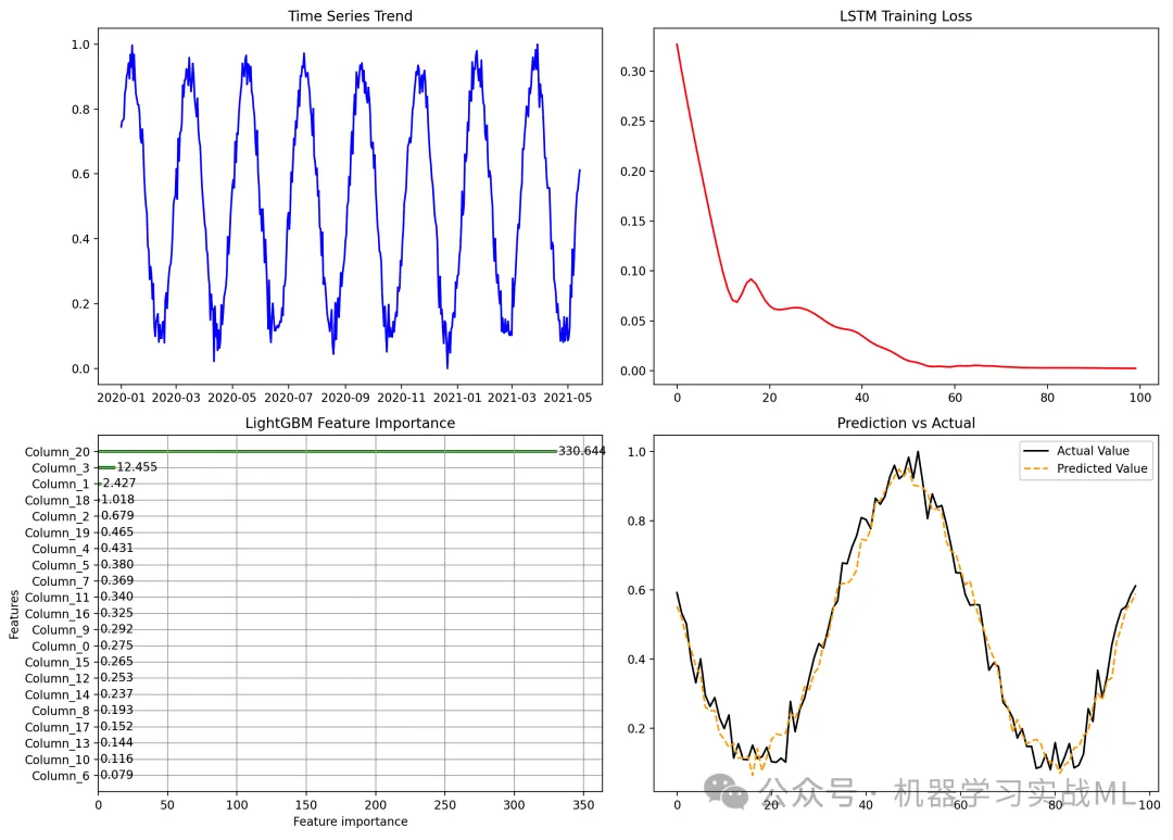
实现了 LSTM 提取特征,再利用 LightGBM 进行时间序列预测,包含:
- 时间序列趋势:观察目标变量的长期变化趋势。
- LSTM 训练损失曲线:展示 LSTM 训练过程的损失变化。
- LightGBM 特征重要性:说明哪些特征贡献最大。
- 预测结果 vs 真实值:直观展示预测的准确性。
)

)


