昇思25天学习打卡营第12天 | ResNet50图像分类
文章目录
- 昇思25天学习打卡营第12天 | ResNet50图像分类
- ResNet网络模型
- 残差网络结构
- Building Block
- Bottleneck
- 训练数据准备
- 训练数据可视化
- 网络构建
- Build Block结构
- Bottleneck结构
- ResNet50网络
- 模型训练与评估
- 训练
- 验证
- 迭代数据集
- 总结
- 打卡
图像分类是最基础的计算机视觉任务,属于有监督学习类别。
ResNet网络模型
在ResNet提出之前,传统的卷积神经网络都是将一系列的卷积层和池化层堆叠而得到的。当网络堆叠到一定的深度时,就会出现退化问题。
ResNet提出了残差网络结构(Residual Network)来减轻退化问题,使得RenNet可以实现较深网络结构的搭建(突破1000层)。
残差网络结构
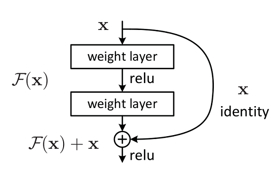
残差网络结构由两个分支构成:
- 主分支:通过堆叠一系列的卷积操作得到
- shortcuts:从输入直接到输出
残差网络结构主要有两种: - Building Block,适用于较浅的ResNet网络,如ResNet18和ResNet34;
- Bottleneck,适用于较深的ResNet网络,如ResNet50、ResNet101和ResNet152;
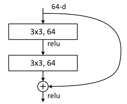
Building Block
Building Block的主分支由两层卷积网络结构:
- 第一层:以输入channel为64为例,首先通过一个 3 × 3 3\times 3 3×3卷积层,然偶通过Batch Normalization层,最后通过 R e L U ReLU ReLU激活函数层,输出channel为64;
- 第二层:输入channel为64,首先通过一层 3 × 3 3\times 3 3×3卷积层,然后通过Batch Normalization层,输出channel为64。
最后主分支输出的特征矩阵与shortcuts输出的特征矩阵相加,通过ReLU激活函数作为Building Block的最后输出。
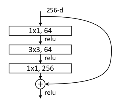
Bottleneck
在输入相同的情况下,Bottleneck结构相比Building Block结构参数数量更少,更适合较深的网络。
该结构的主分支有三层卷积结构,分别为 1 × 1 1\times 1 1×1卷积, 3 × 3 3\times 3 3×3卷积, 1 × 1 1\times 1 1×1卷积,其中 1 × 1 1\times 1 1×1卷积层分别起到降维和升维的作用:
- 第一层:以输入channel为256为例,首先通过数量为64,大小为 1×1的卷积核进行降维,然后通过Batch Normalization层,最后通过Relu激活函数层,其输出channel为64;
- 第二层:通过数量为64,大小为 3×3的卷积核提取特征,然后通过Batch Normalization层,最后通过Relu激活函数层,其输出channel为64;
- 第三层:通过数量为256,大小 1×1的卷积核进行升维,然后通过Batch Normalization层,其输出channel为256。
最后将主分支输出的特征矩阵与shortcuts输出的特征矩阵相加,通过Relu激活函数即为Bottleneck最后的输出。
训练数据准备
CIFAR-10数据集共有60000张 32 × 32 32\times 32 32×32的彩色图像,分为10个类别,每类有6000张图像,数据集一共包含50000张训练图片和10000张评估图片。
from download import downloadurl = "https://mindspore-website.obs.cn-north-4.myhuaweicloud.com/notebook/datasets/cifar-10-binary.tar.gz"download(url, "./datasets-cifar10-bin", kind="tar.gz", replace=True)
使用mindspore.dataset.Cifar10Dataset接口加载数据集,并进行数据增强操作:
import mindspore as ms
import mindspore.dataset as ds
import mindspore.dataset.vision as vision
import mindspore.dataset.transforms as transforms
from mindspore import dtype as mstypedata_dir = "./datasets-cifar10-bin/cifar-10-batches-bin"  # 数据集根目录
batch_size = 256  # 批量大小
image_size = 32  # 训练图像空间大小
workers = 4  # 并行线程个数
num_classes = 10  # 分类数量def create_dataset_cifar10(dataset_dir, usage, resize, batch_size, workers):data_set = ds.Cifar10Dataset(dataset_dir=dataset_dir,usage=usage,num_parallel_workers=workers,shuffle=True)trans = []if usage == "train":trans += [vision.RandomCrop((32, 32), (4, 4, 4, 4)),vision.RandomHorizontalFlip(prob=0.5)]trans += [vision.Resize(resize),vision.Rescale(1.0 / 255.0, 0.0),vision.Normalize([0.4914, 0.4822, 0.4465], [0.2023, 0.1994, 0.2010]),vision.HWC2CHW()]target_trans = transforms.TypeCast(mstype.int32)# 数据映射操作data_set = data_set.map(operations=trans,input_columns='image',num_parallel_workers=workers)data_set = data_set.map(operations=target_trans,input_columns='label',num_parallel_workers=workers)# 批量操作data_set = data_set.batch(batch_size)return data_set# 获取处理后的训练与测试数据集dataset_train = create_dataset_cifar10(dataset_dir=data_dir,usage="train",resize=image_size,batch_size=batch_size,workers=workers)
step_size_train = dataset_train.get_dataset_size()dataset_val = create_dataset_cifar10(dataset_dir=data_dir,usage="test",resize=image_size,batch_size=batch_size,workers=workers)
step_size_val = dataset_val.get_dataset_size()
训练数据可视化
import matplotlib.pyplot as plt
import numpy as npdata_iter = next(dataset_train.create_dict_iterator())images = data_iter["image"].asnumpy()
labels = data_iter["label"].asnumpy()
print(f"Image shape: {images.shape}, Label shape: {labels.shape}")# 训练数据集中,前六张图片所对应的标签
print(f"Labels: {labels[:6]}")classes = []with open(data_dir + "/batches.meta.txt", "r") as f:for line in f:line = line.rstrip()if line:classes.append(line)# 训练数据集的前六张图片
plt.figure()
for i in range(6):plt.subplot(2, 3, i + 1)image_trans = np.transpose(images[i], (1, 2, 0))mean = np.array([0.4914, 0.4822, 0.4465])std = np.array([0.2023, 0.1994, 0.2010])image_trans = std * image_trans + meanimage_trans = np.clip(image_trans, 0, 1)plt.title(f"{classes[labels[i]]}")plt.imshow(image_trans)plt.axis("off")
plt.show()

网络构建
Build Block结构
from typing import Type, Union, List, Optional
import mindspore.nn as nn
from mindspore.common.initializer import Normal# 初始化卷积层与BatchNorm的参数
weight_init = Normal(mean=0, sigma=0.02)
gamma_init = Normal(mean=1, sigma=0.02)class ResidualBlockBase(nn.Cell):expansion: int = 1  # 最后一个卷积核数量与第一个卷积核数量相等def __init__(self, in_channel: int, out_channel: int,stride: int = 1, norm: Optional[nn.Cell] = None,down_sample: Optional[nn.Cell] = None) -> None:super(ResidualBlockBase, self).__init__()if not norm:self.norm = nn.BatchNorm2d(out_channel)else:self.norm = normself.conv1 = nn.Conv2d(in_channel, out_channel,kernel_size=3, stride=stride,weight_init=weight_init)self.conv2 = nn.Conv2d(in_channel, out_channel,kernel_size=3, weight_init=weight_init)self.relu = nn.ReLU()self.down_sample = down_sampledef construct(self, x):"""ResidualBlockBase construct."""identity = x  # shortcuts分支out = self.conv1(x)  # 主分支第一层:3*3卷积层out = self.norm(out)out = self.relu(out)out = self.conv2(out)  # 主分支第二层:3*3卷积层out = self.norm(out)if self.down_sample is not None:identity = self.down_sample(x)out += identity  # 输出为主分支与shortcuts之和out = self.relu(out)return out
Bottleneck结构
class ResidualBlock(nn.Cell):expansion = 4 # 最后一个卷积核的数量是第一个卷积核数量的4倍def __init__(self, in_channel: int, out_channel: int,stride: int = 1, down_sample: Optional[nn.Cell] = None) -> None:super(ResidualBlock, self).__init__()self.conv1 = nn.Conv2d(in_channel, out_channel,kernel_size=1, weight_init=weight_init)self.norm1 = nn.BatchNorm2d(out_channel)self.conv2 = nn.Conv2d(out_channel, out_channel,kernel_size=3, stride=stride,weight_init=weight_init)self.norm2 = nn.BatchNorm2d(out_channel)self.conv3 = nn.Conv2d(out_channel, out_channel * self.expansion,kernel_size=1, weight_init=weight_init)self.norm3 = nn.BatchNorm2d(out_channel * self.expansion)self.relu = nn.ReLU()self.down_sample = down_sampledef construct(self, x):identity = x # shortscuts分支out = self.conv1(x) # 主分支第一层:1*1卷积层out = self.norm1(out)out = self.relu(out)out = self.conv2(out) # 主分支第二层:3*3卷积层out = self.norm2(out)out = self.relu(out)out = self.conv3(out) # 主分支第三层:1*1卷积层out = self.norm3(out)if self.down_sample is not None:identity = self.down_sample(x)out += identity # 输出为主分支与shortcuts之和out = self.relu(out)return out
ResNet50网络
ResNet50网络层结构如下图所示:
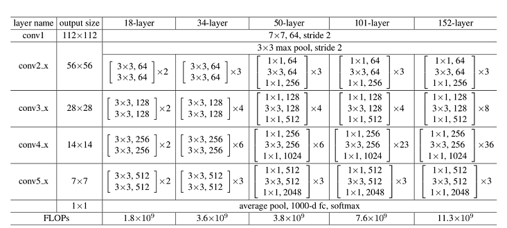
对于输入 224 × 224 224\times 224 224×224彩色图像:
- 通过数量64,卷积核大小 7 × 7 7\times 7 7×7, s t r i d e = 2 stride = 2 stride=2的卷积层conv1,输出图片大小为 112 × 112 112\times 112 112×112,通道为64;
- 通过 3 × 3 3\times 3 3×3的最大下采样池化层,输出输出图片大小为 112 × 112 112\times 112 112×112,通道为64;
- 堆叠4个残差网络块(conv2_x、conv3_x、conv4_x和conv5_x),输出图片大小为 7 × 7 7\times 7 7×7,通道为2048。
- 通过一个平均池化层、全连接层和softmax,得到分类概率。
对于每个残差网络块,如ResNet50的conv2_x,其由3个Bottleneck结构堆叠,每个Bottleneck输入channel为64,输出channel为256.
def make_layer(last_out_channel, block: Type[Union[ResidualBlockBase, ResidualBlock]],channel: int, block_nums: int, stride: int = 1):down_sample = None # shortcuts分支if stride != 1 or last_out_channel != channel * block.expansion:down_sample = nn.SequentialCell([nn.Conv2d(last_out_channel, channel * block.expansion,kernel_size=1, stride=stride, weight_init=weight_init),nn.BatchNorm2d(channel * block.expansion, gamma_init=gamma_init)])layers = []layers.append(block(last_out_channel, channel, stride=stride, down_sample=down_sample))in_channel = channel * block.expansion# 堆叠残差网络for _ in range(1, block_nums):layers.append(block(in_channel, channel))return nn.SequentialCell(layers)from mindspore import load_checkpoint, load_param_into_netclass ResNet(nn.Cell):def __init__(self, block: Type[Union[ResidualBlockBase, ResidualBlock]],layer_nums: List[int], num_classes: int, input_channel: int) -> None:super(ResNet, self).__init__()self.relu = nn.ReLU()# 第一个卷积层,输入channel为3(彩色图像),输出channel为64self.conv1 = nn.Conv2d(3, 64, kernel_size=7, stride=2, weight_init=weight_init)self.norm = nn.BatchNorm2d(64)# 最大池化层,缩小图片的尺寸self.max_pool = nn.MaxPool2d(kernel_size=3, stride=2, pad_mode='same')# 各个残差网络结构块定义self.layer1 = make_layer(64, block, 64, layer_nums[0])self.layer2 = make_layer(64 * block.expansion, block, 128, layer_nums[1], stride=2)self.layer3 = make_layer(128 * block.expansion, block, 256, layer_nums[2], stride=2)self.layer4 = make_layer(256 * block.expansion, block, 512, layer_nums[3], stride=2)# 平均池化层self.avg_pool = nn.AvgPool2d()# flattern层self.flatten = nn.Flatten()# 全连接层self.fc = nn.Dense(in_channels=input_channel, out_channels=num_classes)def construct(self, x):x = self.conv1(x)x = self.norm(x)x = self.relu(x)x = self.max_pool(x)x = self.layer1(x)x = self.layer2(x)x = self.layer3(x)x = self.layer4(x)x = self.avg_pool(x)x = self.flatten(x)x = self.fc(x)return xdef _resnet(model_url: str, block: Type[Union[ResidualBlockBase, ResidualBlock]],layers: List[int], num_classes: int, pretrained: bool, pretrained_ckpt: str,input_channel: int):model = ResNet(block, layers, num_classes, input_channel)if pretrained:# 加载预训练模型download(url=model_url, path=pretrained_ckpt, replace=True)param_dict = load_checkpoint(pretrained_ckpt)load_param_into_net(model, param_dict)return modeldef resnet50(num_classes: int = 1000, pretrained: bool = False):"""ResNet50模型"""resnet50_url = "https://mindspore-website.obs.cn-north-4.myhuaweicloud.com/notebook/models/application/resnet50_224_new.ckpt"resnet50_ckpt = "./LoadPretrainedModel/resnet50_224_new.ckpt"return _resnet(resnet50_url, ResidualBlock, [3, 4, 6, 3], num_classes,pretrained, resnet50_ckpt, 2048)
模型训练与评估
使用ResNet50预训练模型进行微调。调用resnet50构造ResNet50模型,并设置pretrained参数为True,将会自动下载ResNet50预训练模型,并加载预训练模型中的参数到网络中。然后定义优化器和损失函数,逐个epoch打印训练的损失值和评估精度,并保存评估精度最高的ckpt文件。
# 定义ResNet50网络
network = resnet50(pretrained=True)# 全连接层输入层的大小
in_channel = network.fc.in_channels
fc = nn.Dense(in_channels=in_channel, out_channels=10)
# 重置全连接层
network.fc = fc# 设置学习率
num_epochs = 5
lr = nn.cosine_decay_lr(min_lr=0.00001, max_lr=0.001, total_step=step_size_train * num_epochs,step_per_epoch=step_size_train, decay_epoch=num_epochs)
# 定义优化器和损失函数
opt = nn.Momentum(params=network.trainable_params(), learning_rate=lr, momentum=0.9)
loss_fn = nn.SoftmaxCrossEntropyWithLogits(sparse=True, reduction='mean')def forward_fn(inputs, targets):logits = network(inputs)loss = loss_fn(logits, targets)return lossgrad_fn = ms.value_and_grad(forward_fn, None, opt.parameters)def train_step(inputs, targets):loss, grads = grad_fn(inputs, targets)opt(grads)return loss
训练
import os
import mindspore.ops as ops# 创建迭代器
data_loader_train = dataset_train.create_tuple_iterator(num_epochs=num_epochs)
data_loader_val = dataset_val.create_tuple_iterator(num_epochs=num_epochs)# 最佳模型存储路径
best_acc = 0
best_ckpt_dir = "./BestCheckpoint"
best_ckpt_path = "./BestCheckpoint/resnet50-best.ckpt"if not os.path.exists(best_ckpt_dir):os.mkdir(best_ckpt_dir)def train(data_loader, epoch):"""模型训练"""losses = []network.set_train(True)for i, (images, labels) in enumerate(data_loader):loss = train_step(images, labels)if i % 100 == 0 or i == step_size_train - 1:print('Epoch: [%3d/%3d], Steps: [%3d/%3d], Train Loss: [%5.3f]' %(epoch + 1, num_epochs, i + 1, step_size_train, loss))losses.append(loss)return sum(losses) / len(losses)
验证
def evaluate(data_loader):"""模型验证"""network.set_train(False)correct_num = 0.0 # 预测正确个数total_num = 0.0 # 预测总数for images, labels in data_loader:logits = network(images)pred = logits.argmax(axis=1) # 预测结果correct = ops.equal(pred, labels).reshape((-1, ))correct_num += correct.sum().asnumpy()total_num += correct.shape[0]acc = correct_num / total_num # 准确率return acc
迭代数据集
# 开始循环训练
print("Start Training Loop ...")for epoch in range(num_epochs):curr_loss = train(data_loader_train, epoch)curr_acc = evaluate(data_loader_val)print("-" * 50)print("Epoch: [%3d/%3d], Average Train Loss: [%5.3f], Accuracy: [%5.3f]" % (epoch+1, num_epochs, curr_loss, curr_acc))print("-" * 50)# 保存当前预测准确率最高的模型if curr_acc > best_acc:best_acc = curr_accms.save_checkpoint(network, best_ckpt_path)print("=" * 80)
print(f"End of validation the best Accuracy is: {best_acc: 5.3f}, "f"save the best ckpt file in {best_ckpt_path}", flush=True)
总结
这一节中介绍了卷积网络在层数较深的时候会出现退化问题,而ResNet网络中提出的残差网络能比较好的解决这一退化问题。残差网络由两个分支组成,主分支通过堆叠卷积操作得到,而shortcuts分支直接从输入数据得到,对于输入 x x x,得到 F ( x ) + x F(x)+x F(x)+x,然后通过Relu激活函数后输出。此外还介绍了Building Block和Bottlenec两种残差网络结构。
打卡


)


